Forecasting with a CGE model: does it work?

Eleventh Floor, Menzies Building Monash University, Wellington Road CLAYTON Vic 3800 AUSTRALIA

Telephone: from overseas:

(03) 9905 2398, (03) 9905 5112 61 3 9905 2398 or 61 3 9905 5112

Fax:

(03) 9905 2426 61 3 9905 2426

e-mail: impact@buseco.monash.edu.au Internet home page: http//www.monash.edu.au/policy/

Forecasting with a CGE model:

Does it Work?

by

P

ETER

B.

DIXON

Centre of Policy Studies

Monash University

and

M

AUREEN

T.

RIMMER

Centre of Policy Studies

Monash University

General Paper No. G-197 May 2009

ISSN 1 031 9034 ISBN 978 1 921654 04 6

Forecasting with a CGE model: does it work?

by

Peter B. Dixon and Maureen T. Rimmer∗ Centre of Policy Studies, Monash University

May 29, 2009 (revised October 6, 2009)

Abstract

Computable general equilibrium models can be used to generate detailed forecasts of output growth for commodities/industries. The main objective is to provide realistic baselines from which to calculate the effects of policy changes. In this paper, we assess a CGE forecasting method that has been applied in policy analyses in the U.S. and Australia. Using data available up to 1998, we apply the method with the USAGE model to generate “genuine forecasts” for 500 U.S. commodities/industries for the period 1998 to 2005. We then compare these forecasts with actual outcomes and with alternate forecasts derived as extrapolated trends from 1992 to 1998.

JEL: C68; E37; F14; O03

Key words: CGE validation; Forecasting; U.S. CGE

∗

This project was undertaken at the suggestion of Bob Koopman. It has taken a long time. We thank him for his unfailing support and enthusiasm. We also thank: Nick Grossman for expert assistance with the trade data; Bill Powers and Janine Dixon for valuable technical suggestions concerning the

Table of Contents

1. Introduction 1

2. Baseline forecasting with the USAGE model: methodology 2

2.1 Historical simulations 2

2.2 Forecast simulations 3

3. Setting the exogenous variables in the forecast simulation for 1998 to 2005 4

3.1 Macro and energy variables 5

3.2 Technology and consumer preferences: top-level nests 5

3.3 Export 8

3.4 Import prices, tariffs and import/domestic preferences 9

3.5 Other variables 9

4. Measuring forecast performance 9

5. Forecasting performance for 1998 to 2005 10

5.1 Overall performance of the pure forecast 10

5.2 Improving performance by getting the exogenous movements right 13 5.3 How can USAGE forecasts beat or get beaten by trend forecasts? 20

6. Concluding remarks 22

References 25

Tables, Figures and Charts

Figure 2.1 Relationship between Historical and Forecast Simulations 5 Figure 5.1 Sequence of forecast simulations for 1998 to 2005 16 Table 3.1 Percentage movements in macro variables 6 Table 3.2 Percentage movements in energy variables between 1998 and 2005 6 Table 3.3 Shocked technology and preference variables in the 1998-2005

forecast simulation 8

Table 5.1 M coefficients for USAGE forecasts of growth in commodity

outputs between 1998 and 2005 11

Table 5.2 AE coefficients for USAGE forecasts of growth in commodity

outputs between 1998 and 2005 11

Table 5.3 M coefficients for USAGE forecasts of growth in commodity

output between 1998 and 2005 12

Table 5.4 AE coefficients for USAGE forecasts of growth in commodity

outputs between 1998 and 2005 12

Chart 5.1 Actual percentage growth in the outputs of the 503 USAGE

commodities, 1998 to 2005: ranked from lowest to highest 14 Chart 5.2 Percentage forecast errors for commodity outputs 1998-2005:

extrapolated 1992-98 trend versus pure USAGE forecast 14 Chart 5.3 Percentage forecast errors for commodity outputs 1998-2005:

1992-98 trend versus USAGE forecast with truth for macro &

energy variables 17

Chart 5.4 Percentage forecast errors for commodity outputs 1998-2005: 1992-98 trend versus USAGE forecast with truth for macro,

energy and trade variables 17

Chart 5.5 Percentage forecast errors for commodity outputs 1998-2005: 1992-98 trend versus USAGE forecast with truth for macro,

Chart 5.6 Percentage growth in commodity export volumes:

Actual 1998-2005 versus actual 1992-98 18

Chart 5.7 Percentage growth in commodity import volumes:

Actual 1998-2005 versus actual 1992-98 19

Chart 5.8 Percentage forecast errors for selected commodity outputs

1998-2005:extrapolated 1992-98 trend versus pure USAGE forecast 21 Chart 6.1 Percentage growth in commodity outputs:

Actual 1998-2005 versus actual 1992-98 23

1. Introduction

Computable general equilibrium (CGE) models have traditionally been used to answer comparative static or “what if” questions. For example, in the U.S. International Trade Commission’s 2004 report on import restraints (USITC, 2004), the USAGE model1 was used to answer the question: what would happen to output and employment in different industries if all significant import restraints were removed? No attempt was made at forecasting. Literally, the question that USAGE answered was: how different would the structure of the U.S. economy have been in 1998 (the then year of the USAGE database) if there had been no significant import restraints from the way it was with significant import restraints. However, policy makers in 2004 are not interested in alternative pictures of 1998. When they are contemplating reductions in import restraints, they want to know how such a policy would affect a future year, say 2011.

There would be no problem if the best answer to the 2011 question were the same as the answer to the 1998 question. But it is not. While forecasting is difficult and problematic, the 1998 structure of the economy, or even the 2004 structure is not the best guess about the structure in 2011. When we give the economy of 2011 our best forecast, then the results for the effects of policy changes can look quite different from those derived under the implicit assumption that the future structure of the economy is the same as the past.

The importance of the baseline was recognized by the USITC in their 2007 report on import restraints (USITC, 2007). In that report, the USITC applied USAGE to calculate the effects of changes in trade policies as deviations around an explicit USAGE projection of the economy out to 2011, starting from a database for 2005. In this projection, the USITC built in the idea that even without reductions in protection, sensitive industries such as Textiles, Apparel and Sugar are likely to be smaller in 2011 than they were in 2005. Thus, the USITC avoided exaggerating the likely economy-wide effects in 2011 of reductions in import restraints.

The method used by the USITC to generate a baseline was derived from an approach that was first used in policy-oriented CGE analyses in Australia.2 In this paper, we assess the USITC method. Using data available up to 1998 we apply the method to generate forecasts for 1998 to 2005. We then compare these forecasts with outcomes for this period and with alternate forecasts derived as extrapolated trends from 1992 to 1998.

Having made a pure forecast for 1998 to 2005 (that is one using only information available up to 1998) we then conduct a series of forecast simulations in which we successively introduce the ‘truth’ for the movements in different groups of exogenous variables. We start by introducing the actual movements in macro and energy variables (that is we replace the forecast movements with the actual movements). Then we replace forecast movements in trade variables with actual movements. Next we replace forecast movements in technology and preference variables with actual movements. Finally, we set all remaining exogenous variables in the forecast simulation at their actual values. This final simulation must necessarily reproduce actual movements for all

1

USAGE is a dynamic CGE model developed at the Centre of Policy Studies, Monash University, in collaboration with the U.S. International Trade Commission. The theoretical structure of USAGE is similar to that of the MONASH model of Australia (Dixon and Rimmer, 2002). However, in both its theoretical and empirical detail, USAGE goes beyond MONASH. Prominent applications of USAGE by the U.S. International Trade Commission include USITC (2004 and 2007).

2

variables. The aim of the successive simulations is to assess of the importance of different exogenous factors in determining the accuracy of forecasts for outputs by commodity.

The remainder of the paper is organized as follows. Sections 2 and 3 describe the forecasting method and its application in creating forecasts for 1998 to 2005 using only data available up to 1998. Section 4 discusses measures of forecasting performance. Section 5 contains results. Concluding remarks are in section 6.

2. Baseline forecasting with the USAGE model: methodology

In common with the MONASH model of Australia (Dixon and Rimmer, 2002), USAGE is designed for four modes of analysis:

Historical, where we estimate changes in technology, consumer preferences, positions of foreign demand curves for U.S. products and numerous other naturally exogenous trade variables;

Decomposition, where we explain periods of economic history in terms of driving factors such as changes in technology, consumer preferences and trade variables; Forecast, where we derive basecase forecasts for industries, occupations and regions that are consistent with trends from historical simulations and with available expert opinions; and

Policy, where we derive deviations from basecase forecast paths caused by assumed policies.

The focus of this paper is forecasting. However, historical analysis is also relevant because of its role in providing trends for use in forecast simulations.

2.1. Historical simulations

We have completed historical simulations for 1992 to 1998 and 1998 to 2005. These simulations quantify changes in consumer preferences and in several aspects of the technologies used in U.S. industries including: intermediate-input-saving technical change; primary-factor-saving technical change; labor-capital bias in technical change; and import-domestic bias in technical change. They also quantify shifts in foreign demand curves for U.S. exports, foreign supply curves for U.S. imports and several other naturally exogenous international variables mainly concerning foreign assets and liabilities.

In an historical simulation for a particular period, as much information as possible is introduced on movements over the period in prices and quantities for consumption, exports, imports and government spending disaggregated by commodity and on movements in employment, investment and capital stocks disaggregated by industry. Most of these variables are naturally endogenous. However, to give them their historical movements, they must be treated as exogenous variables. Correspondingly, aspects of technology and preferences are endogenized.

The general approach in historical simulations can be understood by reference to the treatment of household consumption. In USAGE, household consumption is explained by equations of the form:

n ,..., 1 i ), i ( com 3 a ) k ( p * ) k , i ( ) q c ( * ) i ( q ) i ( x ₃ k

3 − =ε − +∑ η + = (2.1)

where ) i (

q is the percentage change in the number of households;

c is the percentage change in aggregate expenditure by households; )

k (

p₃ is the percentage change in the price to households of commodity k; a3com(i) is a commodity-i preference variable; and

) i (

ε and η(i,k) are estimates of the expenditure elasticity of demand by households for commodity i and the elasticity of demand for commodity i with respect to changes in the price of k.

In an historical simulation, x3(i), q, c and p3(k) are set exogenously at their observed values for a particular period and preference changes are deduced by allowing (2.1) to be satisfied via endogenous movements in a3com(i). Our historical simulations for 1992 to 1998 and 1998 to 2005 revealed preference changes against [negative a3com(i)s] Tobacco products, Malt beverages Wine and spirits, Bowling centers and Newspapers, and preference changes in favor of [positive a3com(i)s] Boatbuilding, Luggage, Travel trailers, Sporting clubs and Cable TV.

Similarly, technology changes are deduced from an historical simulation by introducing observed changes for output quantities, input quantities and input prices and allowing input-demand equations to be satisfied by endogenous changes in technology variables. Our historical simulations for 1992 to 1998 and 1998 to 2005 revealed: rapid technological progress in the production of Computers and Financial services; slow or negative technological progress in the production of Childcare services and Vet services; significant positive input-using technological change for Computers, Job training and Management services; and significant negative input-using technological change for Glass, Sawmill products and Brick and clay tiles.

2.2. Forecast simulations

The philosophy of forecast simulations is similar to that of historical simulations. In historical simulations we exogenize what is known about the past. In forecast simulations we exogenize what we think we know about the future. Historical simulations are not an attempt to attribute causes to past events. Historical simulations simply reproduce those events. Attributing causation is the role of decomposition simulations in which past events are explained in terms of changes in technology, changes in preferences and changes in other naturally exogenous variables. Forecast simulations are not an attempt to attribute causes to future events. They simply give our “most likely picture” of future events. Attributing causation is the role of policy simulations in which potential future events are explained in terms of changes in naturally exogenous variables, particularly policy variables.

For the past a lot is known about disaggregated versions of naturally endogenous variables (e.g. consumption by commodity). For the future, views about naturally endogenous variables are restricted to a much smaller group, mainly macro variables (e.g. aggregate consumption). For macro variables projections are available from expert forecasting organizations (e.g. the Congressional Budget Office). Because CGE modelers have no particular expertise in macro forecasting, and because CGE models typically omit some factors (e.g. the inventory cycle) that are important in macro forecasting, it is sensible in creating a CGE baseline to use expert macro forecasts.

scalar propensities (e.g. the average propensity to consume is endogenized to accommodate exogenous projections of aggregate consumption). In forecast simulations, vector shocks are applied mainly to naturally exogenous variables (e.g. technical change and preference variables are shocked with trends derived mainly from historical simulations).

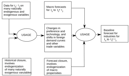
The relationship between historical and forecast simulations is illustrated in Figure 2.1. The current year is denoted by t0, the historical period is t0 - τ1 to t0 and the

forecast period is t0 to t0 + τ2. As can be seen from that figure, baseline forecasts

developed according to USAGE methodology build in considerable data from the past and expert macro opinion for the future.

3. Setting the exogenous variables in the forecast simulation for 1998 to 2005

This section describes the creation of forecast for 1998 to 2005, in which we use only information available up to 1998.

In creating a forecast for 1998 to 2005, we start with a complete dataset (values for every variable) for 1998. Shocks are then applied to exogenous variables to represent movements from their 1998 values to their forecast values for 2005. The exogenous variables receiving non-zero shocks in our 1998-2005 forecast simulation can be partitioned into the following groups:

• Macro and energy variables. As described in sub-section 3.1, the shocks for these variables are derived from forecasts made by U.S. government agencies published in or before 1998.

Figure 2.1 Relationship between Historical and Forecast Simulations

Historical closure, involves

endogenization of many naturally exogenous varuiables

0 t +τ₂ 0 t Macro forecasts for to Changes in preference and technology, and shifts in foreign demand curves and other trade variables Forecast closure, involves endogenization of macro propensities USAGE USAGE Baseline forecast for industries for 0 t +τ₂ 0

t to Data for on

many naturally endogenous and exogenous variables

t -₀ τ1

• International-trade shift variables. These include movements in: foreign demand curves for U.S. products; foreign-currency prices for U.S. imports; tariffs and tariff rate equivalents of quotas; and preferences by households and industries for imported varieties of goods relative to domestic varieties. As described in sub-sections 3.3 and 3.4, the shocks for these variables are derived mainly from extrapolations from the 1992-98 historical simulation.

• Other variables.

3.1 Macro and energy variables

The macro assumptions underlying our forecasts for 1998 to 2005 are shown in the second column of Table 3.1. These forecasts were an amalgam of forecasts made in 1998 by the Congressional Budget Office and other official U.S. organizations. The first and third columns of Table 3.1 show outcomes for 1992-1998 and 1998-2005.

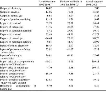
For energy variables, we took the 1998 forecasts from Annual Energy Outlook 1996 published in January 1996 by the Energy Information Administration (EIA) in the U.S. Department of Energy. These forecasts are shown in the second column of Table 3.2. The first and third columns show outcomes, taken from Annual Energy Outlook 2006.

3.2 Technology and consumer preferences: top-level nests

USAGE contains many technology and preference variables. Technology variables in USAGE are predominantly of the input- or output-augmenting/saving type. They are the A variables in production functions of the form:

⎟ ⎟ ⎠ ⎞ ⎜ ⎜ ⎝ ⎛ = mj mj j 1 j 1 nj nj j 1 j 1 j 1 A 1 X ..., , 1 A 1 X ; 0 X * 0 A ..., , 0 X * 0 A F

0 (3.1)

Table 3.1 Percentage movements in macro variables

Actual outcome

1992-1998

Forecast available in 1998 for 1998-05

Actual outcome 1998-2005

Real private consumption 24.13 15.78 28.00

Real investment 60.60 16.43 26.09

Real public consumption 3.99 15.29 19.10

Real exports 47.64 57.32 23.76

Real imports 70.57 46.17 55.12

Real GDP 24.57 15.37 21.64

Aggregate employment 11.92 9.42 7.79

Aggregate capital stock 17.30 20.90 19.49

Ave. nominal wage rate 23.37 25.50 29.94

Consumer price level 11.83 19.02 16.16

Terms of trade 6.46 -0.26 -5.57

Dwelling investment 35.99 18.25 45.36

Table 3.2 Percentage movements in energy variables between 1998 and 2005

Actual outcome 1992-1998

Forecast available in 1998 for 1998-05

Actual outcome 1998-2005

Output of electricity 16.87 0.35 7.06

Output of crude oil -13.06 -9.51 -15.85

Output of natural gas 6.68 16.04 -5.81

Output of petroleum refining 11.45 11.79 9.67

Imports of crude oil 35.39 27.71 16.44

Imports of natural gas 47.46 28.36 37.27

Imports of petroleum refining 8.42 27.59 50.30

Exports of crude oil 23.49 44.79 -72.73

Exports of natural gas -26.48 75.00 368.75

Exports of petroleum refining -9.81 44.79 28.92

Inputs of coal to electricity 16.45 12.07 12.57

Inputs of petroleum refining to electricity

23.92 -46.67 -7.27

Inputs of natural gas to electricity

30.92 61.45 57.07

Import price of crude petroleum relative to GDP deflator

-40.31 12.23 309.23

Import price of natural gas relative to GDP deflator

4.70 2.38 260.89

Price of domestic coal relative to GDP deflator

-19.19 -7.58 21.47

Price of domestic electricity relative to GDP deflator

-13.83 -7.81 19.12

Household consumption of natural gas

ij 0

X is the output of commodity i by industry j; and qj

1

X is the input of commodity or primary factor q to production in j.

A 10 per cent reduction in A0_ij represents 10 per cent output-i-augmenting technical change in

industry j. With a 10 per cent reduction in A0_ij, industry j is able to expand its output of i by 10

per cent with no change in the output of any other commodity and no change in inputs. A 10 per cent reduction in A1_qj represents 10 per cent input-q-saving technical change in industry j. With a 10 per cent reduction in A1_qj, industry j can reduce its input of q by 10 per cent with no change in any other input and no change in outputs. Technology variables in USAGE cover not only current production, but also the use of inputs in creating capital for each industry and the use of margin services in facilitating commodity flows between producers and users.

Preference variables are included in USAGE as A variables in the household utility function. In stylized form, utility is given by

⎟⎟ ⎠ ⎞ ⎜⎜ ⎝ ⎛ = n n 1 1 3 A 3 X ..., , 3 A 3 X U

U (3.2)

where i 3

X is consumption of commodity i.

A 10 per cent reduction in A3_i represents a 10 per cent preference shift against commodity i. With a 10 per cent reduction in A3_i, households can reduce their purchases of i by 10 per cent with no change in any other purchase and no change in utility.

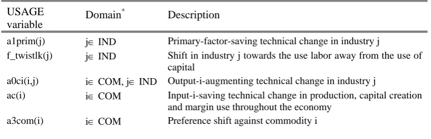
Nearly all of the USAGE technology and preference variables are treated exogenously in the 1998 to 2005 forecast simulation and are given movements (adjusted from 6 years to 7 years) reflecting those that they had, either endogenously or exogenously, in the historical simulation for 1992 to1998.3 Technology and preference variables that were given non-zero shocks in 1998 to 2005 are listed in Table 3.3. The first of these, a1prim(j), imparts a uniform shock in industry j’s production function to the A1 variables referring to primary factors. Biases in industry j’s primary-factor-saving technical change are introduced via f_twistlk(j). The a0ci(i,j)s refer to shocks to the A0 variables in j’s production function. In the historical simulations we have only aggregate data on the use of commodity i as a margin service and as an input to current production and capital creation. Consequently, the historical simulations reveal only a single value for commodity-i-using technical change. This is projected forward from 1998 to 2005 through shocks to the USAGE variable ac(i). The a3com(i)s refer to shocks to the A3 variables in the household utility function.

An important USAGE technology variable that is treated endogenously in the 1998 to 2005 forecast is a1primgen. This is a scalar variable. It imparts a uniform primary-factor-saving technical change across all industries. The role of endogenous movements in a1primgen can be understood in terms of the equations:

3

Table 3.3 Shocked technology and preference variables in the 1998-2005 forecast simulation

USAGE

variable Domain *

Description

a1prim(j) j∈ IND Primary-factor-saving technical change in industry j

f_twistlk(j) j∈ IND Shift in industry j towards the use labor away from the use of capital

a0ci(i,j) i∈ COM, j∈ IND Output-i-augmenting technical change in industry j

ac(i) i∈ COM Input-i-saving technical change in production, capital creation and margin use throughout the economy

a3com(i) i∈ COM Preference shift against commodity i

*

IND is the set of all industries and COM is the set of all commodities.

M X G I C

GDP= + + + − and (3.3)

) L , K ( F * A

GDP= . (3.4)

Equation (3.3) is the GDP identity from the expenditure side and equation (3.4) represents GDP from the supply side as a function of inputs of capital and labor (K and L) and of technology (A). In our forecast for 1998 to 2005, movements in C, I, G, X, M, K and L are given exogenously via the macro scenario in Table 3.1. Thus A must be endogenous. In USAGE, the required degree of freedom for technology is provided by endogenous determination of a1primgen.

3.3 Exports

In slightly stylized form, the export demand equations in USAGE are:

x4(i) = z_world + φ(i)*[p4(i) – p4fn(i) - fep(i)] + feq_gen, (3.5) and

p4fn(i) = pm(i) + f_p4 (i) . (3.6)

In equation (3.5),

x4(i)is the percentage change in foreign demand for U.S. commodity i; z_world is the percentage change in the world activity level (world GDP);

p4(i) is the percentage change in the foreign-currency price of U.S. export product i in foreign countries;

p4fn(i) is the percentage change in the foreign-currency price of foreign commodities that are competitive with U.S. product i in foreign countries;

φ(i) is the foreign elasticity of demand for U.S. product i, treated as a parameter with value -3 for all i; and the

f terms are shifts in the foreign demand curve for U.S. product i. In equation (3.6),

pm(i) is the percentage change in the foreign currency import price of i; and f_p4(i) is a shift term.

Via equation (3.6), we can assume that the movement in the price of commodities that are competitive with U.S. commodity i in foreign countries is the same as that in the price of the relevant imports to the U.S.

Our historical simulation for 1992 to 1998 revealed movements [fep(i)] in foreign demand curves. These are extrapolated in the forecasts for 1998 to 2005 as contributions4 to growth in commodity outputs.

3.4 Import prices, tariffs and import/domestic preferences

In our forecast simulation for 1998 to 2005, we assume for most commodities that the percentage changes in foreign-currency import prices [pm(i)] will be the same (apart from adjustment from 6 years to 7 years) as for the period 1992 to 1998. For various energy prices we use forecasts from the EIA (see subsection 3.1). For tariff rates and the tariff rate equivalents of quotas we assume in the forecasts that there is no change between 1998 and 2005.

The historical simulation for 1992 to 1998 reveals shifts in consumer and industry preferences between imported and domestic varieties of the same good. These are movements in import/domestic ratios beyond those that can be attributed to movements in import/domestic prices. In the 1998 to 2005 forecast we extrapolate the observed 1992-98 shifts as contributions to output growth for each commodity.

3.5. Other variables

In forecast simulations there are numerous exogenous variables apart from those discussed above. These describe: the commodity composition of public-sector demand; required rates of return on investment by industry; tax rates; population; and interest, dividend and revaluation rates applying to U.S. foreign assets and liabilities. For most of these variables we derived our forecasts for 1998 to 2005 as extrapolations of movements between 1992 and 1998. However, for required rates of return on investment we made an exception. These are volatile variables and we doubt that historical movements provide any useful guidance for the future. Thus in forecasting we assumed no change in these variables at the industry level, although we did allow for an overall uniform change to accommodate macro forecasts for wage rates and technology.

4. Measuring forecast performance

In the context of this paper, the first measure of forecast performance that comes to mind is average error (AE) applied to the USAGE forecasts for commodity outputs. AE can be defined as

c

c c

c

1 a

AE * f a 1

100

N ∑

⎛ ⎞ ⎛ ⎞

=_{⎜ ⎟} − _⎜ + _⎟

⎝ ⎠

⎝ ⎠ (4.1)

where

fc is the forecast of the percentage change in the output of commodity c between

1998 and 2005;

ac is the actual percentage change in the output of commodity c between 1998 and

2005; and

N is the number of commodities (503 in the present application of USAGE).

The term for commodity c on the RHS of (4.1) is the gap between the forecast output for commodity c in 2005 and the actual output, expressed a percentage of the actual output. Thus AE is an unweighted average across the 503 USAGE commodities in percentage gaps between forecast levels of commodity outputs and actual levels.

4

If AE turns out to be close to zero, then there is no difficulty in declaring the forecast to be a success. However, as we will see in the next section, the AE values that we obtain seem rather high, e.g. 19 per cent. However, before being disappointed, we should look at what can be done without a model. The most obvious non-model approach is historical trends. On this logic, a performance measure for the USAGE forecasts that builds in a fair comparison is:

c c c c c c c c a

f a 1

100 M

a

h a 1

100 ∑ ∑ ⎛ ⎞ − _⎜ + _⎟ ⎝ ⎠ = ⎛ ⎞ − _⎜ + _⎟ ⎝ ⎠ (4.2) where

hc is the percentage change in the output of commodity c across the historical period,

1992 to 1998, extrapolated to make it apply for a seven-year period rather than a six-year period.

M is the ratio of the average error in the USAGE forecast to the average error in a forecast based on extrapolation. If M = 1, then the USAGE-based forecast is no more or less accurate than a non-model-based forecast generated by trends. If on the other hand, M = 0.7, we can say that by using USAGE we have eliminated 30 per cent of the error involved in simply relying on historical trends.

Variants of (4.1) and (4.2) are

c

c c c

c

a

AE(W) W * f a 1

100

∑ ⎛ ⎞

= − _⎜ + _⎟

⎝ ⎠ , and (4.3)

c

c c c

c

c

c c c

c

a

W * f a 1

100 M(W)

a

W * h a 1

100 ∑ ∑ ⎛ ⎞ − _⎜ + _⎟ ⎝ ⎠ = ⎛ ⎞ − _⎜ + _⎟ ⎝ ⎠ (4.4)

where the W’s are weights. If we are particularly interested in trade issues, for example, we can set Wc as commodity c’s share in U.S. imports or U.S. exports or U.S. total trade.

By setting the W’s in this way, we can test the performance of our model in forecasting activity in trade-oriented sectors of the economy.

5. Forecasting performance for 1998 to 2005

5.1 Overall performance of the pure forecast

Tables 5.1 to 5.4 present results from applying formula (4.3) and (4.4). [Results for formulas (4.1) and (4.2) are the same as those in the first rows of the tables, uniform weights.] In this subsection we consider the results in the first column of the tables, those for pure forecasts. The next subsection considers the results in the other columns.

The rows of the tables show results with different weights (Wc). In row 1, the

error for each commodity is given the same weight (1/Nc). In rows 2, 3 and 4, Wc is the

Table 5.1 M coefficients for USAGE forecasts of growth in commodity outputs between 1998 and 2005

(1) (2) (3) (4) (5)

Identifier Weights Pure

forecast

(1)+ Macro & Energy

(2)+trade & tariffs

(3)+technology & preferences

Actuals for all exog.

1 uniform 0.58 0.54 0.36 0.14 0.0

2 imports 0.56 0.51 0.23 0.14 0.0

3 exports 0.54 0.45 0.26 0.13 0.0

4 imports plus exports 0.55 0.48 0.24 0.14 0.0

5 uniform, merchandise only 0.56 0.51 0.31 0.14 0.0

6 imports, merchandise only 0.55 0.49 0.22 0.13 0.0

7 exports, merchandise only 0.49 0.39 0.25 0.13 0.0

8 imports plus exports,

merchandise only

0.53 0.45 0.23 0.13 0.0

Table 5.2 AE coefficients for USAGE forecasts of growth in commodity outputs between 1998 and 2005

(1) (2) (3) (4) (5)

Identifier Weights Pure

forecast

(1)+ Macro & Energy

(2)+trade & tariffs

(3)+technology & preferences

Actuals for all exog.

1 uniform 18.9 17.7 11.6 4.6 0.0

2 imports 25.3 23.0 10.3 6.2 0.0

3 exports 21.8 18.1 10.4 5.1 0.0

4 imports plus exports 22.7 20.8 10.4 5.7 0.0

5 uniform, merchandise only 21.1 19.2 11.7 5.2 0.0

6 imports, merchandise only 28.3 25.1 11.2 6.9 0.0

7 exports, merchandise only 24.8 19.6 12.3 6.7 0.0

8 imports plus exports,

merchandise only

27.0 23.0 11.6 6.8 0.0

Table 5.3 M coefficients for USAGE forecasts of growth in commodity output between 1998 and 2005

(1) (2) (3) (4) (5)

Identifier Weights Pure

forecast

(1)+ Macro & Energy

(2)+technology & preferences

(3)+trade & tariffs

Actuals for all exog.

1 uniform 0.58 0.54 0.35 0.14 0.0

2 imports 0.56 0.51 0.38 0.14 0.0

3 exports 0.54 0.45 0.35 0.13 0.0

4 imports plus exports 0.55 0.48 0.37 0.14 0.0

5 uniform, merchandise only 0.56 0.51 0.35 0.14 0.0

6 imports, merchandise only 0.55 0.49 0.36 0.13 0.0

7 exports, merchandise only 0.49 0.39 0.26 0.13 0.0

8 imports plus exports,

merchandise only

0.53 0.45 0.32 0.13 0.0

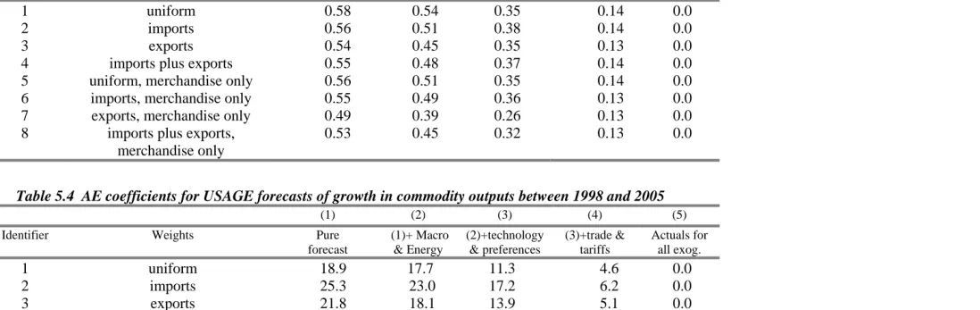
Table 5.4 AE coefficients for USAGE forecasts of growth in commodity outputs between 1998 and 2005

(1) (2) (3) (4) (5)

Identifier Weights Pure

forecast

(1)+ Macro & Energy

(2)+technology & preferences

(3)+trade & tariffs

Actuals for all exog.

1 uniform 18.9 17.7 11.3 4.6 0.0

2 imports 25.3 23.0 17.2 6.2 0.0

3 exports 21.8 18.1 13.9 5.1 0.0

4 imports plus exports 22.7 20.8 15.7 5.7 0.0

5 uniform, merchandise only 21.1 19.2 13.1 5.2 0.0

6 imports, merchandise only 28.3 25.1 18.4 6.9 0.0

7 exports, merchandise only 24.8 19.6 13.0 6.7 0.0

8 imports plus exports,

merchandise only

13

What conclusions should we draw from the tables for the pure forecasts? At first glance the AE results seem large. As indicated by GDP growth (Table 3.1), output growth for the average industry between 1998 and 2005 was about 21.64 per cent. Yet the forecast error for a typical industry is 18.9 per cent (row 1, column 1, Tables 5.2 and 5.4). This would be a disastrously large average error if all industries had actual growth rates in a tight band around 21.64. But they did not. As shown in Chart 5.1, the actual growth rates were spread over the range -66 (for slippers) to 218 (for computer peripheral equipment). Only 151 out of the 503 USAGE commodities exhibited output growth within 10 percentage points of the average.

The M coefficient gives a more optimistic view of the USAGE forecasts than obtained from AE. When every commodity is treated as equally important the M coefficient indicates that USAGE reduces the forecast error by 42 per cent relative to a simple non-modeling extrapolation approach (row 1, column 1, Tables 5.1 and 5.3). The difference between the AE and M perspectives for measuring forecast performance is illustrated in Chart 5.2. The chart shows for each of the 503 USAGE commodities the trend forecast error, h_c−a / 1 a 100_c

(

)

(

)

c c c

f −a / 1 a 100+ , on the vertical axis. With the AE perspective we consider only the

values on the vertical axis: AE with uniform weights is a simple average of these values. With the M perspective, we consider the values on both axes. Because the bulk of the points in Chart 5.2 are below the 45-degree line, the M perspective tells us that the USAGE forecasts have comfortably outperformed a simple trend forecasts.

With a trade emphasis (rows 2-4 and 6-8, column 1, Tables 5.1 and 5.3), the M measure gives the USAGE forecasts an even better score than when every commodity is treated as equally important. For example, when merchandise export weights (row 7) are used, USAGE eliminates 51 per cent of the forecast error that would be made with a simple extrapolation approach.

While the M coefficient falls when weighting schemes emphasizing trade are adopted, AE rises. For example, in column 1 of Tables 5.1 and 5.2, as we go from uniform weights to import merchandise weights, M falls from 0.58 to 0.55 whereas AE rises from 18.9 to 28.3. Similarly, as we go from uniform weights to export merchandise weights, M falls from 0.58 to 0.49 whereas AE rises from 18.9 to 24.8. Outputs of import-competing and export-oriented commodities are hard to forecast. As will be shown in the next subsection, growth rates in imports and exports by commodity in the forecast period (1998-2005) bear little relationship to growth rates in the historical period (1992-98). Thus, high average errors in forecasting outputs of trade exposed commodities are to be expected. It is reassuring that for these commodities the USAGE forecasting method, building in considerable structural detail, offers particularly strong improvement over simple trends.

5.2 Improving performance by getting the exogenous movements right

14

Chart 5.1 Actual percentage growth in the outputs of the 503 USAGE commodities, 1998 to 2005: ranked from lowest to highest

-100 -50 0 50 100 150 200 250

0 100 200 300 400 500 600

Chart 5.2 Percentage forecast errors for commodity outputs 1998-2005: extrapolated 1992-98 trend versus pure USAGE forecast

0 50 100 150 200 250

0 50 100 150 200 250

USAGE forecast errors

Trend forecast errors M(uniform) = 0.58

AE(uniform) = 18.9

Asbestos products

15

replace the forecast values and in the fourth column we introduce the true values for the movements in technology and preference variables. Column (5) introduces the true values for movements in all remaining exogenous variables. Visually, the improvements in forecasting performance from successive introduction of the truth for exogenous variables can be seen from the movement of the points in Charts 5.2 to 5.5 towards the horizontal axis.

Tables 5.3 and 5.4 introduce the true values for the exogenous variables in a different order from that in Tables 5.1 and 5.2. By comparing Tables 5.3 and 5.4 with 5.1 and 5.2, we can see that the contributions of accurate trade forecasts to the USAGE forecasting performance on commodity outputs does not depend strongly on whether or not the technology/preference forecasts are accurate. Similarly, the contribution of accurate technology/preference forecasts does not depend strongly on whether or not the trade forecasts are accurate. This means that we can draw unambiguous conclusions about the value of improving trade forecasts on the one hand and technology/preference forecasts on the other.

Comparison between columns (1) and (2) of the tables shows that the availability in 1998 of accurate macro and energy forecasts for the period 1998 to 2005 would have generated a useful improvement in our ability to forecast commodity outputs. With uniform weights, the M coefficient is reduced from 0.58 to 0.54 while the AE coefficient falls 18.9 to 17.7. Accurate macro and energy forecasts have their greatest impact on the USAGE forecasting performance when performance is measured with export weights (rows 3 and 7). For example, if export merchandise weights are used, the M coefficient improves from 0.49 to 0.39 and the AE coefficient drops from 24.8 to 19.6. USAGE forecasts for export commodities were particularly poorly informed by the 1998 macro forecast. As can be seen from Table 3.1, in the macro forecast adopted in USAGE, aggregate exports increased by 57.32 per cent. The true outcome was an increase of only 23.76 per cent. Telling USAGE about the 23.76 per cent significantly improves the model’s ability to forecast output growth for heavily exported commodities.

A major improvement in the USAGE forecasting performance comes when the model is given the truth about exogenous trade and tariff variables. In Tables 5.1 and 5.2 (the left-hand sequence in Figure 5.1), M(uniform) improves from 0.54 to 0.36 and AE(uniform) falls from 17.7 to 11.6 when we introduce “the truth” for these variables. Similarly, in Tables 5.3 and 5.4 (the right-hand sequence), introduction of the truth for trade variables improves M(uniform) by over 20 points, from 0.35 to 0.14. The importance of trade and tariff variables is perhaps surprising because for most commodities import shares in the U.S. market and export shares in output are quite small: 64 per cent of USAGE commodities in 1998 had import shares of less than 15 per cent and 73 per cent of USAGE commodities had export shares of less than 15 per cent.

16

Figure 5.1 Sequence of forecast simulations for 1998 to 2005

Pure forecast

Replace macro and energy forecasts with the truth

Pure forecast

Replace trade shift forecasts

with the truth Replace technology & preference_{forecasts with the truth}

Replace other exogenous forecasts with the truth

Replace trade shift forecasts with the truth Replace technology & preference

forecasts with the truth

Replace other exogenous forecasts with the truth M(uniform) = 0.58

AE(uniform) = 18.9

M(uniform) = 0.54 AE(uniform) = 17.7

M(uniform) = 0.36 AE(uniform) = 11.6

M(uniform) = 0.35 AE(uniform) = 11.3

M(uniform) = 0.14 AE(uniform) = 4.6

M(uniform) = 0.14 AE(uniform) = 4.6

M(uniform) =0.00 AE(uniform) = 0.0

17

Chart 5.3 Percentage forecast errors for commodity outputs 1998-2005: 1992-98 trend versus USAGE forecast with truth for macro & energy variables

0 50 100 150 200 250

0 50 100 150 200 250

USAGE forecast errors

Trend forecast errors M(uniform)= 0.54

AE(uniform) = 17.7

Chart 5.4 Percentage forecast errors for commodity outputs 1998-2005:

1992-98 trend versus USAGE forecast with truth for macro, energy and trade variables

0 50 100 150 200 250

0 50 100 150 200 250

USAGE forecast errors

Trend forecast errors M(uniform)= 0.36

18

Chart 5.5 Percentage forecast errors for commodity outputs 1998-2005: 1992-98 trend versus USAGE forecast with truth for macro, energy, trade and

technology & preference variables

0 50 100 150 200 250

0 50 100 150 200 250

USAGE forecast errors

Trend forecast errors M(uniform)= 0.14

AE(uniform) = 4.6

Chart 5.6 Percentage growth in commodity export volumes: Actual 1998-2005 versus actual 1992-98

y = -0.2097x + 45.467 R2 _{= 0.03}

-200 0 200 400 600 800 1000

-200 -100 0 100 200 300 400 500 600

Exports for 1998-2005

19

Chart 5.7 Percentage growth in commodity import volumes: Actual 1998-2005 versus actual 1992-98

y = 0.1412x + 39.697 R2 _{= 0.0677}

-200 -100 0 100 200 300 400 500 600 700

-200 0 200 400 600 800 1000 1200

Imports for 1998-2005

Imports for 1992-1998

Getting the movements right in the technology and preference variables makes a similar contribution to forecasting performance as the introduction of accurate forecasts for exogenous trade variables. The introduction of the truth for technology and preference variables reduces M(uniform) by 22 points in Table 5.1 (from 0.36 to 0.14) and 19 points in Table 5.3 (from 0.54 to 0.35).

20

5.3 How can USAGE forecasts beat or get beaten by trend forecasts?

USAGE forecasts incorporate trend assumptions for nearly all technology, preference and trade-shift variables. Movements in these variables are major determinants of changes in the commodity composition of U.S. output. A reasonable question therefore is how does USAGE generate forecasts for commodity outputs that are distinctly different from trend forecasts.

Part of the answer is that the USAGE takes in macro and energy forecasts that need not reflect trends. These forecasts push many of the USAGE commodity forecasts away from trends. We consider some examples.

New residential construction, additions and alterations (USAGE commodities 32-35)

Most of the sales of these commodities are to investment in Ownership of Dwellings. The 1998-2005 USAGE forecasts for the output of the residential construction commodities was determined mainly by the macro forecast for dwelling investment (18.25 per cent, Table 3.1). For the historical period 1992 to 1998, output growth for residential construction was determined mainly by actual growth for dwelling investment (35.99 per cent, Table 3.1). Thus, our USAGE forecasts for residential construction imply considerably weaker growth for 1998 to 2005 than that given by an extrapolation of the trend. In this particular case, we would have been better off with extrapolation of the trend. The outcome for 1998 to 2005 for dwelling investment (45.36 per cent) was much closer to an extrapolation of the trend than the forecast available in 1998. This explains why the residential construction dots in Chart 5.8 lie above the 45-degree line.

Computers and office machinery (USAGE commodities 317-20)

These commodities are used widely across industries in capital creation. Therefore aggregate investment is an important determinant of their output growth. Between 1992 and 1998 aggregate investment grew by 60.6 per cent (Table 3.1). In 1998, aggregate investment was forecast to grow by 16.43 per cent between 1998 and 2005. On this basis, USAGE generated growth forecasts for output of computers and office equipment over the period 1998 to 2005 that were considerably lower than the trend growth rates from the period 1992 to 1998. The outcome for 1998 to 2005 for aggregate investment (26.09 per cent) was much closer to the 1998 forecast than to the historical trend (26.09 per cent compared with 73.79 per cent5). Consequently, as illustrated in Chart 5.8, the USAGE forecasts for computers and office machinery easily beat the trend forecasts.

Electricity (USAGE commodity 411)

This is a commodity in which the incorporation of expert energy forecasts for the period 1998 to 2005 enabled USAGE to outperform the forecast based on the 1992-98 trend. As can be seen from Table 3.2, growth in electricity output between 1992 and 1998 was 16.87 per cent, giving a trend forecast for 1998 to 2005 of 19.95 per cent. The expert forecast incorporated into USAGE for the period 1998 to 2005 was 0.35 per cent. This is closer to the truth (7.06 per cent) than is the trend forecast (Chat 5.8).

While the macro and energy forecasts are important in explaining how USAGE generates commodity forecasts that depart from the trend, they are not the whole story. To establish that there are other factors we consider two further examples.

21

Chart 5.8 Percentage forecast errors for selected commodity outputs 1998-2005: extrapolated 1992-98 trend versus pure USAGE forecast

0 50 100 150 200 250

0 50 100 150 200 250

Residential construction

Electricity

Computer and office equipment USAGE forecast errors

Trend forecast errors

Railroad equipment (USAGE commodity 362)

As can be seen from Chart 5.2, for this commodity USAGE strongly out-performs trend (the point for Railroad equipment is far below the 45-degree line). The USAGE error is 12 per cent whereas the trend error is 110 per cent. While not shown in the chart, the actual growth in the output of Railroad equipment was -9.3 per cent. The USAGE and trend forecasts are 1.5 per cent and 90 per cent.

More than half the sales of railroad equipment are to investment in Railroad services. Over the period 1992-98, investment in railroad services rose by 156 per cent. This imparted strong growth to output of Railroad equipment, about 74 per cent between 1992 and 1998, leading to the trend forecast of 90 per cent growth for 1998-2005.

In the USAGE simulation for 1992 to 1998, Railroad services arrives in 1998 with copious capital and a quite low rate of return. With only moderate output growth predicted for Railroad services, USAGE translated the low rate of return into weak investment for the period 1998 to 2005. This led to the USAGE forecast, which turned out to be correct, of negligible growth in the output of Railroad equipment.

Asbestos products (USAGE commodity 233)

22

Most of the sales of this commodity are to the transport equipment industries (aircraft, motor vehicle parts, etc). In 1992, there were also significant exports. Between 1992 and 1998, exports almost completely disappeared. In the USAGE simulation for 1992-98, there was a sharp inward movement of the foreign demand curve. At the same time there was strong growth in imports. Output of the commodity between 1992 and 1998 fell by 12 per cent. However, with strong import growth and apparent diversion of exports back to the domestic market, the USAGE simulation for 1992-98 showed fast growth in supplies on the domestic market relative demands by the transport-equipment industries. In these circumstances, the model implied that during the period 1992 to 1998 there was asbestos-using technical change in the transport equipment industries (positive ac(i) for i= 233). In the forecast for 1998 to 2005, this asbestos-using technical change was projected forward. The inward movement in the export demand curve was also projected forward, but with exports in 1998 at approximately zero, this did not significantly affect the forecast output for Asbestos products. The transport equipment industries in the 1998-2005 forecast showed moderate growth. Combined with the projected asbestos-using technical change, this was enough to give erroneously good prospects for Asbestos products in the USAGE forecasts.

The obvious problem with the USAGE forecast in this case is the assumption that asbestos-using technical change was positive in the period 1998-2005. Even in 1998 it would almost certainly have been possible to foresee negative asbestos-using technical change. It is also perhaps surprising that we found positive asbestos-using technical change for the period 1992-98. This brings into question our data for 1992 to 1998. We have checked the trade data thoroughly and found no problem. We may now need to revisit the output data for the period.

6. Concluding remarks

Perhaps the most common reaction of policy makers/advisors when confronted with results from a detailed computable general equilibrium (CGE) model is: “how do I know these results are accurate?” This is a difficult question to answer. So far, the best answers that CGE modelers have been able to provide are in the form of back-of-the-envelope justifications. However, what is really needed is a statistical demonstration that CGE models can produce usefully accurate predictions of:

(1) changes in the commodity/industrial composition of economic activity under business-as-usual assumptions; and

(2) the effects on macro and industry variables of changes in trade and other policies.

In the context of (1), by “usefully accurate” we mean predictions that are better than those obtained by simple trends. In the context of (2), we mean predictions that are better than those obtained by surveys of opinions of industry experts.

In this paper we have started work on issue (1). Predicting output movements at the 500 commodity level is not an easy job. As can be seen from Chart 6.1, past movements are a very imperfect guide to future movements. Encouragingly, we have found that USAGE output forecasts at the 500-commodity level comfortably outperform trends. On the other hand, average errors for these forecasts seem alarmingly high.

23

Chart 6.1 Percentage growth in commodity outputs: Actual 1998-2005 versus actual 1992-98

y = 0.4522x - 6.7934 R2 _{= 0.4072}

-100 -50 0 50 100 150 200 250

-100 -50 0 50 100 150 200 250 300 350 400 450

Outputs for 1998-2005

Outputs for 1992-1998

Chart 6.2. Imports of Butter from 1992 to 2005 ($million)

0 20 40 60 80 100 120 140

24

undertook an audit of the trade data for 1992, 1998 and 2005. We also examined the trade data for the intervening years and experimented with forecasts for 1998 to 2005 that relied on a 1992-1998 historical simulation incorporating smoothed versions of growth in export and import volumes. This work yielded little improvement in the USAGE forecasting performance. We are forced to the conclusion that at the 500-commodity level U.S. trade is volatile. For example, Chart 6.2 shows annual imports of Butter over the period 1992 to 2005 varying between approximately 0 and $130 million. To improve USAGE forecasting performance it is apparent that the underlying causes of volatile trade behavior must be understood so that informed opinions can be built into the forecasts concerning future movements. This suggests an approach in which preliminary forecasts are made and then tested in discussions with industry experts. The U.S. International Trade Commission and the Departments of Commerce and Agriculture, three of the agencies that use USAGE, seem well placed to provide feedback on institutional and technological factors that should be taken into account in creating forecasts at a detailed level.

In future research we hope to investigate issue (2): the accuracy of CGE models in predicting the effects of changes in trade (and other) policies. This issue is even more difficult than assessing the validity of a basecase forecast. The problem is that during any period in which an economy is adjusting to a change in trade policies, other factors will also be operating. This point was not adequately addressed in the often-cited validation exercise by Kehoe (2005). In that exercise, Kehoe assesses the performance of various models in predicting the effects of NAFTA. He notes that the model of Brown, Deardorff and Stern predicted that NAFTA would increase Mexican exports by 50.8%. Over the period 1988 to 1999, Mexican exports went up by 140.6 per cent. Kehoe invites us to draw the conclusion that Brown et al. strongly underestimated the effects of NAFTA. However, what about all the other factors that affected Mexican trade volumes over these 10 years?

25

References:

Bureau of Labor Statistics, BLS (2008), “National employment matrices”, available at

http://www.bls.gov/emp/empocc2.htm .

Dixon, P.B., J. Menon and M.T. Rimmer (2000), “Changes in technology and preferences: a general equilibrium explanation of rapid growth in trade”, Australian Economic Papers, Vol. 39(1), March, pp.33 – 55.

Dixon, P.B., M.T. Rimmer (2002), Dynamic General Equilibrium Modelling for Forecasting and Policy: a Practical Guide and Documentation of MONASH,

Contributions to Economic Analysis 256, North-Holland Publishing Company, Amsterdam, pp.xiv+338.

Dixon, P.B. and M.T. Rimmer (2006) “Employment by occupation and industry, 2004 and 2014: Technical documentation”, pp. 35, Available from the Centre of Policy Studies website at http://www.monash.edu.au/policy/ftp/techusage1.pdf .

Energy Information Administration (1996), Annual Energy Output 1996, with projections to 2015, Office of Integrated Analysis and Forecasting, U.S. Department of Energy, Washington DC, January, pp.221.

Energy Information Administration (2006), Annual Energy Output 2006, with projections to 2030, Office of Integrated Analysis and Forecasting, U.S. Department of Energy, Washington DC, February, pp.275.

Feenstra, R.C. (1994), “New Product Varieties and the Measurement of International Prices”,

The American Economic Review, 84(1), March, pp. 157-77.

Harris, R.G. (1984), “Applied General Equilibrium Analysis of Small Open Economies with Scale Economies and Imperfect Competition”, American Economic Review, 74(5), pp. 1016-32.

Harrison, W.J., J.M. Horridge and K.R. Pearson (2000), “Decomposing simulation results with respect to exogenous shocks”, Computational Economics, Vol. 15, pp. 227–49. Kehoe, T.J. (2005) “An Evaluation of the Performance of Applied General Equilibrium

Models of the Impact of NAFTA,” in Timothy J. Kehoe, T.N. Srinivasan, and John Whalley, editors, Frontiers in Applied General Equilibrium Modeling: Essays in Honor of Herbert Scarf, Cambridge University Press, pp. 341–77.

Krueger, A.O. (1974), “The Political Economy of the Rent-seeking Society”, American Economic Review, 64, June, pp. 291-303.

Leibenstein, H. (1966), “Allocative efficiency versus X-efficiency”, American Economic Review, 56, June, pp. 392-415.

Melitz, M.J. (2003), “The Impact of Trade on Intra-Industry Reallocations and Aggregate Industry Productivity”, Econometrica, 71(6), November, pp. 1695-1725.

United States International Trade Commission (2004), The Economic Effects of Significant U.S. Import Restraints: Fourth Update 2004, Investigation No. 332-325, Publication 3701, June.