Characterization of Neutron Detection Systems with
Confidence via Statistical Parameter Correction
Phillip Boone
Nucsafe, Inc. Oak Ridge, USA [email protected]
Abstract—Neutron detection systems utilize statistical alarm techniques where a measured false alarm rate (FAR) can vary drastically from the FAR predicted by a theoretical model. The ability to set an alarm threshold that results in a practically controlled FAR is crucial to characterize detector sensitivity with both accuracy and precision. A generalized and automated method is presented to statistically evaluate FAR performance by assuming that the FAR itself is not deterministic, but a normal stochastic process over a specific parameter to be corrected that will hereafter be referred to as thecorrection. In this manner, a specific correction results in not only a point estimate of FAR, but also a confidence interval. The central objective is focused exclusively on characterization assuming that experiments are executed in a tightly controlled environment so that an accurate comparison is enabled across detectors. Once a correction is calculated, the estimated FAR is only assumed accurate in a similar environment for sensitivity evaluation. Initially, the calcu-lated correction factor was used to compare FARs across various distributions including normal, corrected normal, Poisson, and a simplified normal distribution. Later verification data sets were used to empirically demonstrate the rate of containment of measured confidence coefficients using two detectors of different technology. A second application uses the correction method to improve the signal-to-noise ratio metric to agree more with dynamic sensitivity results. Finally, a third application studies the effect of altering the duration of background acquisition on FAR performance.
I. INTRODUCTION
B
Y partitioning a notably large set of background data into potentially thousands of mutually exclusive periods, a distinct alarm threshold can be calculated using a specific correction and statistics on an individual background period. By applying this distinct threshold, a single alarm rate sample can be calculated over the remaining background data. Each subsequent background period is used likewise to create addi-tional alarm rate samples for the entire data set. A maximum likelihood problem is formulated in section II-D1 assuming that a detector’s false alarm rate (FAR) is a normal random process of correction. Using numerical optimization in section II-E, a first-order search is utilized to determine a correction to meet a target FAR.False alarm performance of the corrected model is compared to three statistical models in section III-C. In section IV, additional background data is gathered to verify that the estimated correction results in the desired FAR with statistical confidence.
In section V three neutron detection systems demonstrate that the signal-to-noise ratio (SNR) metric may result in a theoretical sensitivity that contradicts sensitivity measured with a more rigorous dynamic test [1] according to American National Standards Institute (ANSI). Section V-A2 introduces a correction to SNR and section V-C demonstrates that the correction results in a sensitivity that agrees more with the rigorous ANSI test.
Section VI studies the effect of reducing the duration of background acquisition from 5 minutes down to a minute. As a result, system sensitivity decreased via the increase in critical value required to meet a target FAR. In addition, the overall precision of FAR drastically decreased via the estimated increase in standard deviation of FAR by a factor of 28.
In the context of the experiments performed, FAR is simply a scaled version of significance level, critical value indicates a specific alarm threshold, and standard critical value represents the number of standard deviations above the mean for an alarm threshold. FAR is used in place of significance level for convenience when presenting measured false alarm rates.
II. STATISTICALMODEL
A. Data Collection Periods
1) Large Experimental Set of Data: Assume that count rate samples for a neutron radiation detector under natural ambient background conditions follow a normal distribution with random variable D ⇠ N(µD, σ2D) and a realization of
ND random samples is the vectorD~ ,[D1, . . . , DND] T.
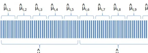
2) Background Partitions of Data: These samples are partitioned into NP B non-overlapping background periods of length NB with the i-th period defined as B~i ,
⇥
DNB(i−1)+1, . . . , DNB(i−1)+NB
⇤T
, [Bi,1, . . . , Bi,NB] T
withi2 {1,2,3, . . . , NP B}.
For each background periodithe statistic that is a minimum
variance unbiased estimator (MVUE) of meanµD is
ˆ
µB,i, 1
NB NB
X
j=1
Bi,j
For each background periodithe statistic that is a MVUE
Fig. 1. Example Data Partitions :ND= 80Samples Partitioned intoNP B=
2 Background Periods ofNB = 40Samples and NP I = 10Integration Periods ofNI= 8Samples
ˆ
σi2, 1
NB−1 NB
X
j=1
(Bi,j−µD)2
The number of samples NB should be chosen as large as possible within system initialization in a known environment without artificial sources.
3) Integration Partitions of Data: The samples in vector
~
D are partitioned again intoNP I << NP B non-overlapping integration periods of lengthNI with the i-th period defined as
~
Ii , ⇥DNI(i−1)+1, . . . , DNI(i−1)+NI
⇤T
, [Ii,1, . . . , Ii,NI] T
withi2 {1,2, . . . , NP I}.
For each periodi the statistic that’s a MVUE of meanµD is
ˆ
µI,i, 1
NI NI
X
j=1
Ii,j
The number of samplesNI is typically chosen to optimize system detection sensitivity for a given source strength and speed.
B. Determine the Theoretical Parameters of a Hypothesis Test Since it can be shown that the test statistic, a linear combi-nation of normal samples, also follows a normal distribution according toµˆI,i⇠ N(µD,σ
2 D
NI), if a one-sided hypothesis test is used then either one of the following choices are possible:
1) Null Hypothesis H0 (radiation is background) a) µˆI,i=µD
2) Alternate Hypothesis H1 (radiation is significantly higher than background)
a) µˆI,i> µD
The critical region of statistic µˆI,i is the region where background radiation is determined to erroneously contain an artificial source (H0 is rejected) and is defined for some constantZ¯↵>0such that
Ci,
⇢
ˆ
µI,i: ˆµI,i> µD+�Z¯↵�pσD
NI
�
(1)
A desired significance level ↵ 2 [0,1] together with the probabilityPH0 of the error region ofH0 constrain a specific solution for constantZ¯↵ according to the equation
PH0(Ci) =↵ (2)
1) Determining a Value for the Standard Critical Value Constant: The standardized test statistic for the i-th period of an integration partition is
Zi, ˆ
µI,i−µD
⇣
σD
p
NI
⌘
and the critical region Ci can be rewritten in terms of the probability of a standard normal distribution (or the cumulative distribution function (Z)) as
Ci,�Zi:P�Zi>Z¯↵�=↵ ={Zi : 1− (Zi) =↵}
where the thresholdZ¯↵, referred to as the standard critical value of the hypothesis test, and corresponding significance level↵can be looked up in a standard normal Z table.
2) Critical Value of the Hypothesis Test: Once the standard critical valueZ¯↵of the standard normal distribution is found, the corresponding critical valueµ¯I,i for the statisticµˆI,i is
¯
µI,i=µD+�Z¯↵�
σD p
NI
(3)
3) Verification of Significance Level: In order to facilitate calculating the value of the error probability in (2), an indicator function1µ(µ) :R! {0,1}is defined as
1µ(µ) =
(
1 when µ > µD+�Z¯↵�pσND I 0 when µµD+�Z¯↵�pσNDI where the expected value
E[1µ(ˆµI,i)] =PH0(Ci) =↵
can be estimated using a sample mean of1µ(ˆµI,i)where
ˆ
↵= 1
NP I NXP I
i=1
1µ(ˆµI,i) (4)
C. Determine the Practical Significance Level of a Hypothesis Test
Note that in section II-B the population mean µD and variance σ2
D of a detector are not known exactly. Therefore, assume that a background period of sufficient length NB is used so thatµˆB,i ⇡µD and ˆσi2 ⇡σD2 are substituted in the formulas of the previous section.
1) Execution of a Very Large Number of Experiments via Background Partitions: Typically, when a user performs a false alarm test using a radiation detector the user programs a standard critical value, a single background period is acquired, statistics are performed resulting in an alarm threshold, and this threshold is applied using a live system for a long duration in order to verify a specified FAR.
Instead, if a large numberNDof data samples are recorded and if these samples are partitioned as in II-A, then thresh-olds can be calculated and a false alarm experiment can be performed in post-processing for every possible background period in the entire data set. Also, if the theoretical standard
Fig. 2. Standard Critical Value
critical value Z¯↵ results in a measured significance level that doesn’t agree with the theoretical significance ↵ within
acceptable tolerance, then adjusted standard critical values can be used to iterate through the whole process again.
Furthermore, significance level estimates↵ˆcan be computed for each background and statistics can be calculated on the resulting set to obtain realistic false alarm performance metrics across backgrounds.
2) Verification of Significance Level using Empirical Data: The indicator function defined in II-B3 is redefined using the j-th actual background parameter estimates as 1µ,j(µ) :R! {0,1} according to
1µ,j(µ) =
(
1 when µ >µˆB,j+�Z¯↵�pσˆNj I 0 when µµˆB,j+�Z¯↵�pσˆNj
I
where the corresponding estimated significance level for the j-th background period is
ˆ
↵j= 1
NP I NXP I
i=1
1µ,j(ˆµI,i) (5)
Theorem 1 (Unique Significance): For a one sided upper hypothesis test, if significance level↵is written as a function
of standard critical value Z↵ in the form↵(Z↵) :R![0,1] then the function is strictly decreasing over the domain of the function as illustrated in Fig.2. Therefore, given a unique significance level ↵0 2 [0,1] there exists a corresponding unique standard critical value Z↵0.
3) Experimental Error: Assume that the theoretical stan-dard critical value Z¯↵ does not result exactly in the desired significance level ↵ due to experimental data not fitting the
model exactly, but insteadZ¯↵results in the significance value ˜
↵. The significance level experimental error is then defined as
✏↵,↵˜−↵
Assume that if experimental data approximately retain the property of Theorem 1, then there exists a unique experimental standard critical valueZˆ↵that results in the theoretical signif-icance level↵within tolerable precision. The standard critical value experimental error is then defined as
✏Z ,Z¯↵−Zˆ↵
4) Random Variable of an Experimental Standard Crit-ical Value: Assume that the significance level estimates
{↵ˆj:j2 {1, . . . , NP B}} are a realization of NP B random samples from a random variable with a standard critical value
ˆ
Z↵ that results in the ideal significance level ↵. Samples are assumed to approximately follow a normal distribution [2][pp.216] for sufficiently largeNP B according to
ˆ
↵j⇠ N˙ �↵, σ2↵
�
(6) 5) Practical Significance Level Estimate: Therefore, the sample mean of↵ˆj is the MVUE of significance level
ˆ
µ↵, 1
NP B NXP B
j=1 ˆ
↵j (7)
The sample variance of ↵ˆj is the MVUE of significance level variance
ˆ
σ2 ↵,
1
NP B−1 NXP B
j=1
( ˆ↵j−µˆ↵)2 (8)
D. Determine the Practical Standard Critical Value of a Hypothesis Test
Since samples of ↵ˆj are assumed to approximately follow a normal distribution with mean ↵ and variance σ2
↵, the probability density function (PDF) is
f( ˆ↵j) = 1
σ↵ p
2⇡exp (
−( ˆ↵j−↵)2 2σ2
↵
)
(9)
1) Maximum Likelihood Estimate of Standard Critical Value: The only quantity in (9) that is a function of standard critical valueZ↵ is ↵ˆj, which can be thought of as either a continuous-time stochastic process [3] over parameterZ↵ or a random variable over the family of PDFs [2] indexed on the parameterZ↵ written as↵ˆj(Z↵)when used in the likelihood functions.
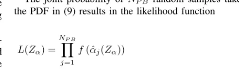
The joint probability of NP B random samples taken from the PDF in (9) results in the likelihood function
L(Z↵) = NYP B
j=1
f( ˆ↵j(Z↵))
= 1
σNP B ↵ (2⇡)
NP B 2
exp
(
−PNP B
j=1 ( ˆ↵j(Z↵)−↵)2 2σ2
↵
)
Fig. 1. Example Data Partitions :ND= 80Samples Partitioned intoNP B=
2 Background Periods ofNB = 40Samples and NP I = 10Integration Periods ofNI= 8Samples
ˆ
σi2, 1
NB−1 NB
X
j=1
(Bi,j−µD)2
The number of samples NB should be chosen as large as possible within system initialization in a known environment without artificial sources.
3) Integration Partitions of Data: The samples in vector
~
D are partitioned again intoNP I << NP B non-overlapping integration periods of lengthNI with the i-th period defined as
~
Ii , ⇥DNI(i−1)+1, . . . , DNI(i−1)+NI
⇤T
, [Ii,1, . . . , Ii,NI] T
withi2 {1,2, . . . , NP I}.
For each periodi the statistic that’s a MVUE of meanµD is
ˆ
µI,i, 1
NI NI
X
j=1
Ii,j
The number of samplesNI is typically chosen to optimize system detection sensitivity for a given source strength and speed.
B. Determine the Theoretical Parameters of a Hypothesis Test Since it can be shown that the test statistic, a linear combi-nation of normal samples, also follows a normal distribution according toµˆI,i⇠ N(µD,σ
2 D
NI), if a one-sided hypothesis test is used then either one of the following choices are possible:
1) Null HypothesisH0 (radiation is background) a) µˆI,i=µD
2) Alternate Hypothesis H1 (radiation is significantly higher than background)
a) µˆI,i> µD
The critical region of statistic µˆI,i is the region where background radiation is determined to erroneously contain an artificial source (H0 is rejected) and is defined for some constantZ¯↵>0 such that
Ci,
⇢
ˆ
µI,i: ˆµI,i> µD+�Z¯↵�pσD
NI
�
(1)
A desired significance level ↵ 2 [0,1] together with the probabilityPH0 of the error region ofH0 constrain a specific solution for constantZ¯↵ according to the equation
PH0(Ci) =↵ (2)
1) Determining a Value for the Standard Critical Value Constant: The standardized test statistic for the i-th period of an integration partition is
Zi, ˆ
µI,i−µD
⇣
σD
p
NI
⌘
and the critical region Ci can be rewritten in terms of the probability of a standard normal distribution (or the cumulative distribution function (Z)) as
Ci,�Zi:P�Zi>Z¯↵�=↵ ={Zi: 1− (Zi) =↵}
where the thresholdZ¯↵, referred to as the standard critical value of the hypothesis test, and corresponding significance level↵can be looked up in a standard normal Z table.
2) Critical Value of the Hypothesis Test: Once the standard critical valueZ¯↵of the standard normal distribution is found, the corresponding critical valueµ¯I,i for the statisticµˆI,i is
¯
µI,i=µD+�Z¯↵�
σD p
NI
(3)
3) Verification of Significance Level: In order to facilitate calculating the value of the error probability in (2), an indicator function1µ(µ) :R! {0,1} is defined as
1µ(µ) =
(
1 when µ > µD+�Z¯↵�pσND I 0 when µµD+�Z¯↵�pσNDI where the expected value
E[1µ(ˆµI,i)] =PH0(Ci) =↵
can be estimated using a sample mean of1µ(ˆµI,i)where
ˆ
↵= 1
NP I NXP I
i=1
1µ(ˆµI,i) (4)
C. Determine the Practical Significance Level of a Hypothesis Test
Note that in section II-B the population mean µD and variance σ2
D of a detector are not known exactly. Therefore, assume that a background period of sufficient length NB is used so thatµˆB,i ⇡µD and ˆσi2 ⇡σD2 are substituted in the formulas of the previous section.
1) Execution of a Very Large Number of Experiments via Background Partitions: Typically, when a user performs a false alarm test using a radiation detector the user programs a standard critical value, a single background period is acquired, statistics are performed resulting in an alarm threshold, and this threshold is applied using a live system for a long duration in order to verify a specified FAR.
Instead, if a large numberNDof data samples are recorded and if these samples are partitioned as in II-A, then thresh-olds can be calculated and a false alarm experiment can be performed in post-processing for every possible background period in the entire data set. Also, if the theoretical standard
Fig. 2. Standard Critical Value
critical value Z¯↵ results in a measured significance level that doesn’t agree with the theoretical significance ↵ within
acceptable tolerance, then adjusted standard critical values can be used to iterate through the whole process again.
Furthermore, significance level estimates↵ˆcan be computed for each background and statistics can be calculated on the resulting set to obtain realistic false alarm performance metrics across backgrounds.
2) Verification of Significance Level using Empirical Data: The indicator function defined in II-B3 is redefined using the j-th actual background parameter estimates as 1µ,j(µ) :R! {0,1} according to
1µ,j(µ) =
(
1 when µ >µˆB,j+�Z¯↵�pˆσNj I 0 when µµˆB,j+�Z¯↵�pˆσNj
I
where the corresponding estimated significance level for the j-th background period is
ˆ
↵j = 1
NP I NP I
X
i=1
1µ,j(ˆµI,i) (5)
Theorem 1 (Unique Significance): For a one sided upper hypothesis test, if significance level↵is written as a function
of standard critical value Z↵ in the form ↵(Z↵) :R![0,1] then the function is strictly decreasing over the domain of the function as illustrated in Fig.2. Therefore, given a unique significance level ↵0 2 [0,1] there exists a corresponding unique standard critical value Z↵0.
3) Experimental Error: Assume that the theoretical stan-dard critical value Z¯↵ does not result exactly in the desired significance level ↵ due to experimental data not fitting the
model exactly, but insteadZ¯↵results in the significance value ˜
↵. The significance level experimental error is then defined as
✏↵,↵˜−↵
Assume that if experimental data approximately retain the property of Theorem 1, then there exists a unique experimental standard critical valueZˆ↵that results in the theoretical signif-icance level↵within tolerable precision. The standard critical value experimental error is then defined as
✏Z,Z¯↵−Zˆ↵
4) Random Variable of an Experimental Standard Crit-ical Value: Assume that the significance level estimates
{↵ˆj:j2 {1, . . . , NP B}} are a realization of NP B random samples from a random variable with a standard critical value
ˆ
Z↵ that results in the ideal significance level ↵. Samples are assumed to approximately follow a normal distribution [2][pp.216] for sufficiently largeNP B according to
ˆ
↵j⇠ N˙ �↵, σ2↵
�
(6) 5) Practical Significance Level Estimate: Therefore, the sample mean of↵ˆj is the MVUE of significance level
ˆ
µ↵, 1
NP B NXP B
j=1 ˆ
↵j (7)
The sample variance of ↵ˆj is the MVUE of significance level variance
ˆ
σ2 ↵,
1
NP B−1 NXP B
j=1
(ˆ↵j−µˆ↵)2 (8)
D. Determine the Practical Standard Critical Value of a Hypothesis Test
Since samples of ↵ˆj are assumed to approximately follow a normal distribution with mean ↵ and variance σ2
↵, the probability density function (PDF) is
f(ˆ↵j) = 1
σ↵ p
2⇡exp (
−(ˆ↵j−↵)2 2σ2
↵
)
(9)
1) Maximum Likelihood Estimate of Standard Critical Value: The only quantity in (9) that is a function of standard critical valueZ↵ is ↵ˆj, which can be thought of as either a continuous-time stochastic process [3] over parameterZ↵ or a random variable over the family of PDFs [2] indexed on the parameterZ↵ written as↵ˆj(Z↵)when used in the likelihood functions.
The joint probability of NP B random samples taken from the PDF in (9) results in the likelihood function
L(Z↵) = NYP B
j=1
f( ˆ↵j(Z↵))
= 1
σNP B ↵ (2⇡)
NP B 2
exp
(
−PNP B
j=1 (ˆ↵j(Z↵)−↵)2 2σ2
↵
)
Fig. 3. Solution to the Cost Function
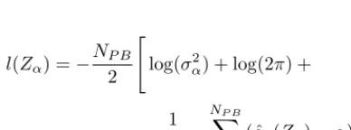
l(Z↵) =−NP B 2
"
log(σ↵2) + log(2⇡) +
1
NP Bσ↵2 NXP B
j=1
(ˆ↵j(Z↵)−↵)2
3 5
Therefore the maximum likelihood estimate of standard critical value is
ˆ
Z↵= arg max Z↵
{l(Z↵)} (10)
E. Optimization Problem Formulation
1) Cost Function: In order to facilitate computation of the likelihood function in (10), all constants independent of Z↵ are eliminated and the negative sign is removed resulting in the following minimization cost function
C(Z↵) = NXP B
j=1
(ˆ↵j(Z↵)−↵)2 (11)
Therefore, the maximum likelihood estimate of (10) is equivalent to minimizing the mean squared error of signifi-cance level↵over standard critical value.
2) Optimization Problem: Using the cost function from (11) in a minimization problem results in the following op-timization problem formulation:
ˆ
Z↵= arg min Z↵
{C(Z↵)}
= arg min Z↵
8 < :
NXP B
j=1
( ˆ↵j(Z↵)−↵)2
9 =
; (12)
3) Optimization Problem Solver: The optimization problem formulated by (12) can be solved using various first order numerical methods, but care must be taken to use a method that is tolerant of noise as illustrated by the solution in Fig.3. In this case, the problem was solved via simulated annealing [4].
F. Generalization of Parameter Correction
The upper hypothesis test utilized normal samples
{µˆI,i:i2 {1, . . . , NP I}} while adjusting the parameter Z↵ to yield a target theoretical significance↵. However, the model
can be made even more flexible by slightly altering definitions including the indicator function in (5). Instead letµ2Rbe a measurable random variable that follows all axioms of proba-bility with the indicator function1µ,j(µ, j, ✓↵) :R! {0,1} where j is a set of statistics on background period j and the parameter✓↵2Ris the target parameter to correct. The indicator function must also be a simple inequality for an upper hypothesis test, ↵ˆj must be approximately normal according to (6), and experimental samples must approximately adhere to Theorem 1. In this case, a much more flexible framework results allowing modification to other system factors such as distribution, correction parameter✓↵, sampling techniques as in section III-B, or another system parameter as in section VI. As factors are adjusted the impact on measured FAR performance valuesµˆ↵ andσˆ↵2 could be evaluated.
III. ERRORANALYSIS USING ANEUTRONDETECTOR
A. Theoretical Probability Distribution vs. Detector Probabil-ity Histogram
In order to qualitatively illustrate the disparity between model and detector data, in Fig.4 a histogram was created for neutron data and scaled theoretical PDFs were overlaid for the normal models. Curie’s criteria was used where variance is assumed equal to the sample mean of data [5][pp.75]. Mat-lab’s histogram function was used with the ”Normalization” parameter set to ”probability” in order to create a probability mass function (PMF). Both PDFs were scaled to have the same maximum value as the PMF. Not only is the histogram data highly discretized but the overall shape does not match either normal model at lower count rates.
B. Correlated Sampling
During problem formulation in section II-A the term ”ran-dom samples” was used to describe theND number of data samples acquired. This is a fundamental assumption often referred to as a set of independent, identically-distributed samples of data. The integration samples as defined in sec-tion II-A3 follow this convensec-tion of sampling. However, the neutron detector data acquired are not sampled independently with non-overlapping segments, but in a temporally correlated and overlapping manner with a slightly different definition of I~i , ⇥D(i
−NI)+1, . . . , D(i−NI)+NI
⇤T
, [Ii,1, . . . , Ii,NI] T
withi2 {NI, NI + 1, . . . , ND}. In other words, every detec-tor sample inD~ starting with number NI is processed as an
average over a rolling buffer where at each iteration the oldest
Fig. 4. Qualitative Probability Comparison
sample is discarded from the beginning and a new sample is inserted to the end. Using this method of sampling is likely a significant contributing factor to the discrepancy between the theoretical standard critical value Z¯↵ and the practical value
ˆ
Z↵.
If independent sampling were performed as originally de-fined the sample rate would be decimated by a factor ofNI. This would result in under sampling where a neutron detector could miss a moving source at sufficient speed that would have been otherwise detected using correlated sampling. Correlated sampling allows the increased sensitivity of averaging periods while retaining the sample rate.
1) Alternate Alarm Definition to Compensate for Correla-tion: A single outlier DO in D~ will persist in the NI −1 correlated samples before andNI−1correlated samples after
DO. Correlated samples µˆI,O−NI+1 through µˆI,O+NI+1 all contain the outlier DO. When processing false alarms for a set of data this is evident when false alarms themselves are observed as temporally correlated.
Consequently, when counting alarms all alarms that occur within a distance of NI −1 samples of another alarm are counted as a single alarm event. The simple heuristic is employed where all correlated samples are first compared as normal to the thresholdµ¯I,jfor the j-th background period and each alarm index is appended to a list. Alarms are processed in sequential order. Assuming that the i-th sample is an alarm then if any alarm exists after the i-th sample in the interval [ˆµI,i+1, . . . ,µˆI,i+NI−1] then the i-th alarm is removed from the alarm set. The same heuristic continues at the subsequent alarm. The whole process is repeated for all background periods.
The alarm heuristic described is incorporated into a class that is used for all presented false alarm measurements of correlated samples.
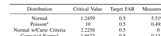
TABLE I
FALSEALARMRATE(per hour)
Distribution Critical Value Target FAR Measured FAR
Normal 1.2459 0.5 5.5195
Poissona 10 0.5 0.4952
Normal w/Curie Criteria 2.2258 0.5 0 Corrected Normal 1.6673 0.5 0.1311
C. Theoretical Model Significance vs. Measured False Alarm Rates
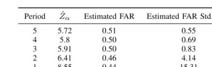
In order to demonstrate the discrepancy between theoretical and measured significance levels, several theoretical models were evaluated. For convenience estimated significance levels were scaled to false alarm rates measured per hour. An 8 segment neutron detector was used to collect 68 hours of data with a sample period of 0.2 seconds, an integration period of 4 seconds, and a background period using the first 5 minutes of data. The requisite statistics for each model were computed on a single background period. The resulting critical values were employed on integrated samples using a similar hypothesis test of section II-B and compensated according to section III-B1. Each distribution was configured with the theoretical critical value to meet a target FAR of 0.5 alarms per hour.
Refer to the results compiled in Table I according to distribution. Since a Poisson model is a discrete distribution of natural numbers, measurements of count rates included in the correlated sampling of III-B are not possible. In this case the unprocessed integer counts were used at the 0.2 second sampling interval. Again, results include a normal model assuming the Curie criteria [5][pp.75]. The last entry labeled ”Corrected Normal” uses a corrected standard critical value that was estimated using the theory developed in this paper. The value Z¯↵ = 4.0309 that results in a false alarm every 2 hours was corrected toZˆ↵= 5.7235.
The results in Table I indicate that the statistical model with the closest FAR to the desired rate is actually a Poisson distribution. However, justification for correlated sampling becomes apparent when the resulting thresholds are all placed on the same scale in the critical value column. The Poisson threshold is approximately six times that of the corrected normal rendering the Poisson model relatively insensitive.
IV. STATISTICALVERIFICATION OFFALSEALARMRATE USINGEMPIRICALDATA
In this section the statistical model of section II is applied to hundreds of background periods using a single data set referred to as the training data. A statistical inference is made during training concerning FAR performance and the training data is set aside. Verification of FAR utilizes a large number of individual false alarm tests [1][pp.17] each of duration 10 hours where the verification library consists of over 1000 hours
Fig. 3. Solution to the Cost Function
l(Z↵) =−NP B 2
"
log(σ↵2) + log(2⇡) +
1
NP Bσ↵2 NXP B
j=1
(ˆ↵j(Z↵)−↵)2
3 5
Therefore the maximum likelihood estimate of standard critical value is
ˆ
Z↵= arg max Z↵
{l(Z↵)} (10)
E. Optimization Problem Formulation
1) Cost Function: In order to facilitate computation of the likelihood function in (10), all constants independent of Z↵ are eliminated and the negative sign is removed resulting in the following minimization cost function
C(Z↵) = NXP B
j=1
(ˆ↵j(Z↵)−↵)2 (11)
Therefore, the maximum likelihood estimate of (10) is equivalent to minimizing the mean squared error of signifi-cance level↵over standard critical value.
2) Optimization Problem: Using the cost function from (11) in a minimization problem results in the following op-timization problem formulation:
ˆ
Z↵= arg min Z↵
{C(Z↵)}
= arg min Z↵
8 < :
NXP B
j=1
( ˆ↵j(Z↵)−↵)2
9 =
; (12)
3) Optimization Problem Solver: The optimization problem formulated by (12) can be solved using various first order numerical methods, but care must be taken to use a method that is tolerant of noise as illustrated by the solution in Fig.3. In this case, the problem was solved via simulated annealing [4].
F. Generalization of Parameter Correction
The upper hypothesis test utilized normal samples
{µˆI,i:i2 {1, . . . , NP I}} while adjusting the parameter Z↵ to yield a target theoretical significance↵. However, the model
can be made even more flexible by slightly altering definitions including the indicator function in (5). Instead letµ2Rbe a measurable random variable that follows all axioms of proba-bility with the indicator function1µ,j(µ, j, ✓↵) :R! {0,1} where j is a set of statistics on background period j and the parameter✓↵2R is the target parameter to correct. The indicator function must also be a simple inequality for an upper hypothesis test, ↵ˆj must be approximately normal according to (6), and experimental samples must approximately adhere to Theorem 1. In this case, a much more flexible framework results allowing modification to other system factors such as distribution, correction parameter✓↵, sampling techniques as in section III-B, or another system parameter as in section VI. As factors are adjusted the impact on measured FAR performance valuesµˆ↵ andσˆ↵2 could be evaluated.
III. ERRORANALYSIS USING ANEUTRONDETECTOR
A. Theoretical Probability Distribution vs. Detector Probabil-ity Histogram
In order to qualitatively illustrate the disparity between model and detector data, in Fig.4 a histogram was created for neutron data and scaled theoretical PDFs were overlaid for the normal models. Curie’s criteria was used where variance is assumed equal to the sample mean of data [5][pp.75]. Mat-lab’s histogram function was used with the ”Normalization” parameter set to ”probability” in order to create a probability mass function (PMF). Both PDFs were scaled to have the same maximum value as the PMF. Not only is the histogram data highly discretized but the overall shape does not match either normal model at lower count rates.
B. Correlated Sampling
During problem formulation in section II-A the term ”ran-dom samples” was used to describe the ND number of data samples acquired. This is a fundamental assumption often referred to as a set of independent, identically-distributed samples of data. The integration samples as defined in sec-tion II-A3 follow this convensec-tion of sampling. However, the neutron detector data acquired are not sampled independently with non-overlapping segments, but in a temporally correlated and overlapping manner with a slightly different definition of I~i , ⇥D(i
−NI)+1, . . . , D(i−NI)+NI
⇤T
, [Ii,1, . . . , Ii,NI] T
withi2 {NI, NI + 1, . . . , ND}. In other words, every detec-tor sample inD~ starting with number NI is processed as an
average over a rolling buffer where at each iteration the oldest
Fig. 4. Qualitative Probability Comparison
sample is discarded from the beginning and a new sample is inserted to the end. Using this method of sampling is likely a significant contributing factor to the discrepancy between the theoretical standard critical value Z¯↵ and the practical value
ˆ
Z↵.
If independent sampling were performed as originally de-fined the sample rate would be decimated by a factor ofNI. This would result in under sampling where a neutron detector could miss a moving source at sufficient speed that would have been otherwise detected using correlated sampling. Correlated sampling allows the increased sensitivity of averaging periods while retaining the sample rate.
1) Alternate Alarm Definition to Compensate for Correla-tion: A single outlier DO in D~ will persist in the NI −1 correlated samples before andNI−1correlated samples after
DO. Correlated samples µˆI,O−NI+1 through µˆI,O+NI+1 all contain the outlier DO. When processing false alarms for a set of data this is evident when false alarms themselves are observed as temporally correlated.
Consequently, when counting alarms all alarms that occur within a distance of NI −1 samples of another alarm are counted as a single alarm event. The simple heuristic is employed where all correlated samples are first compared as normal to the thresholdµ¯I,jfor the j-th background period and each alarm index is appended to a list. Alarms are processed in sequential order. Assuming that the i-th sample is an alarm then if any alarm exists after the i-th sample in the interval [ˆµI,i+1, . . . ,µˆI,i+NI−1] then the i-th alarm is removed from the alarm set. The same heuristic continues at the subsequent alarm. The whole process is repeated for all background periods.
The alarm heuristic described is incorporated into a class that is used for all presented false alarm measurements of correlated samples.
TABLE I
FALSEALARMRATE(per hour)
Distribution Critical Value Target FAR Measured FAR
Normal 1.2459 0.5 5.5195
Poissona 10 0.5 0.4952
Normal w/Curie Criteria 2.2258 0.5 0 Corrected Normal 1.6673 0.5 0.1311
C. Theoretical Model Significance vs. Measured False Alarm Rates
In order to demonstrate the discrepancy between theoretical and measured significance levels, several theoretical models were evaluated. For convenience estimated significance levels were scaled to false alarm rates measured per hour. An 8 segment neutron detector was used to collect 68 hours of data with a sample period of 0.2 seconds, an integration period of 4 seconds, and a background period using the first 5 minutes of data. The requisite statistics for each model were computed on a single background period. The resulting critical values were employed on integrated samples using a similar hypothesis test of section II-B and compensated according to section III-B1. Each distribution was configured with the theoretical critical value to meet a target FAR of 0.5 alarms per hour.
Refer to the results compiled in Table I according to distribution. Since a Poisson model is a discrete distribution of natural numbers, measurements of count rates included in the correlated sampling of III-B are not possible. In this case the unprocessed integer counts were used at the 0.2 second sampling interval. Again, results include a normal model assuming the Curie criteria [5][pp.75]. The last entry labeled ”Corrected Normal” uses a corrected standard critical value that was estimated using the theory developed in this paper. The value Z¯↵ = 4.0309 that results in a false alarm every 2 hours was corrected toZˆ↵= 5.7235.
The results in Table I indicate that the statistical model with the closest FAR to the desired rate is actually a Poisson distribution. However, justification for correlated sampling becomes apparent when the resulting thresholds are all placed on the same scale in the critical value column. The Poisson threshold is approximately six times that of the corrected normal rendering the Poisson model relatively insensitive.
IV. STATISTICALVERIFICATION OFFALSEALARMRATE USINGEMPIRICALDATA
In this section the statistical model of section II is applied to hundreds of background periods using a single data set referred to as the training data. A statistical inference is made during training concerning FAR performance and the training data is set aside. Verification of FAR utilizes a large number of individual false alarm tests [1][pp.17] each of duration 10 hours where the verification library consists of over 1000 hours
of background data per scintillating detector for both a6Li op-tical fiber detector and a Li6coated waveguide detector. Using the statistics estimated during training, confidence intervals were constructed at various coefficients and applied across all verification false alarm tests.
In this section several common experimental procedures are followed. Data is acquired with a sample period of 0.2 seconds, an integration period of 4 seconds, and a background period of 5 minutes. Again, the standard critical value is tuned to meet a target FAR of 0.5 alarms per hour.
A. Confidence Interval using Training Data
Each training data set is acquired such that the number of samples ND results in about 70 hours of data to estimate a correctedZˆ↵ in tandem with the FAR performance statistics ˆ
µ↵andσˆ↵ of section II-C5.
Instead of using the training statistic µˆ↵ over NP B back-ground periods, the target statistic↵ˆjover a single background is used in verification to estimate a confidence interval that models an individual ANSI false alarm experiment [1][pp.17]. The standardized statistic for ↵ˆj is Zj , ↵ˆjσˆ−↵µˆ↵ where the corresponding standard critical value isZ¯↵/2, confidence coefficient is (1 −↵) for ↵ 2 [0,1], and probability of containment is
1−↵=P ✓
−Z¯↵/2< ˆ
↵j−µˆ↵ ˆ
σ↵ < ¯
Z↵/2
◆
(13)
Note that the critical value Z¯↵/2 can be looked up in a standard normal Z table accounting for a two-sided test while
¯
Z↵in (2) uses a single-sided hypothesis test. A realization of a confidence interval [2][pp.216] of FAR for a specific training set is
�
ˆ
↵l,↵ˆu�,�µˆ
↵−�Z¯↵/2�σˆ↵,µˆ↵+�Z¯↵/2�ˆσ↵� (14) and is tested for accuracy via the verification data set described next.
B. Containment of Verification Data
Verification data is segmented into background periods and processed like training data as in section II except thatZˆ↵,µˆ↵, andσˆ↵were already calculated via training data. Each verifi-cation data set is acquired such that the number of samplesND results in exactly 10 hours of data. For a given verification data set and j-th background period,↵ˆj is calculated according to (5) usingZˆ↵from training while the selected verification data set is used to calculate both background statistics µˆB,j and ˆ
σj. The value ↵ˆj is tested to determine if contained within the interval in (14). All verification data sets are processed similarly for the j-th background period. In this manner a measured confidence coefficient is calculated as a simple decimal fraction of successful containment. In order to account for background variation, a confidence coefficient is calculated for every possible background period in addition to the j-th and the result is averaged.µ¨↵ is the sample mean and ¨σ↵2 is the sample variance of ↵ˆj over every background period and every verification data set.
TABLE II
COATEDDETECTORTRAININGDATASETS
Hours 68.7 71.5 71.8 71.9 71.4 72.4 72.1 95.1
ˆ
µD 0.24 0.22 0.23 0.22 0.23 0.22 0.22 0.24
ˆ
σD 0.25 0.24 0.24 0.24 0.24 0.24 0.24 0.25
ˆ
Z↵ 5.70 5.74 5.83 5.77 5.75 5.68 5.83 5.67
ˆ
µ↵ 0.5 0.49 0.49 0.51 0.51 0.5 0.5 0.5
ˆ
σ↵ 0.58 0.55 0.57 0.62 0.62 0.58 0.54 0.61
ˆ
↵l -0.63 -0.58 -0.62 -0.71 -0.70 -0.64 -0.56 -0.69
ˆ
↵u 1.63 1.56 1.61 1.73 1.72 1.63 1.56 1.69
TABLE III
COATEDDETECTORVERIFICATIONRESULTS FOREACHTRAININGDATA SET
Ver. Sets µ¨↵ σ¨↵ 85% 90% 92.5% 95% 97.5% 99% 128 0.52 0.63 87.6 89.8 91.8 94.0 95.1 96.3 127 0.48 0.60 86.5 89.2 90.2 92.3 94.8 95.8 127 0.40 0.54 92.6 93.6 94.9 95.6 96.4 97.9 127 0.46 0.58 91.8 93.5 94.6 95.5 97.5 98.6 127 0.48 0.61 88.8 92.2 93.0 94.6 95.9 98 127 0.53 0.66 86.7 89.4 91.2 92.5 94.1 96.3 127 0.42 0.56 89.5 91.2 92.8 94.2 96.2 96.8 125 0.54 0.66 86.6 88.4 91.2 92.3 95.8 97.6
TABLE IV
COATEDDETECTORVERIFICATIONRESULTS OVER ALLTRAININGDATA SETS
Statistic ↵ˆj 85% 90% 92.5% 95% 97.5% 99% Sample Mean 0.48 88.8 90.9 92.5 93.9 95.7 97.2 Sample Std. 0.61 3.34 2.90 2.53 2.24 1.90 1.64
TABLE V
FIBERDETECTORTRAININGDATASETS
Hours 67.8 69.7 71.5 71.8 71.9 71.4 72.4 72.1
ˆ
µD 2.28 2.30 2.26 2.28 2.27 2.26 2.25 2.24
ˆ
σD 0.81 0.82 0.81 0.81 0.81 0.81 0.80 0.80
ˆ
Z↵ 4.66 4.80 4.71 4.59 4.66 4.59 4.63 4.58
ˆ
µ↵ 0.5 0.5 0.5 0.5 0.5 0.5 0.5 0.5
ˆ
σ↵ 0.35 0.30 0.31 0.41 0.36 0.44 0.41 0.39
ˆ
↵l -0.18 -0.09 -0.10 -0.30 -0.20 -0.36 -0.30 -0.27
ˆ
↵u 1.18 1.10 1.10 1.29 1.21 1.36 1.30 1.26
TABLE VI
FIBERDETECTORVERIFICATIONRESULTS FOR EACHTRAININGDATA SET
Ver. Sets µ¨↵ σ¨↵ 85% 90% 92.5% 95% 97.5% 99% 125 0.49 0.41 87.6 90.8 92.8 92.8 94.7 96.1 125 0.35 0.30 85.7 85.7 97.0 97.0 97.3 98.1 125 0.44 0.37 84.3 93.3 93.3 95.1 95.1 96.3 125 0.58 0.46 86.5 88.3 91.2 91.2 95.4 96.2 125 0.49 0.40 90.9 90.9 92.7 94.4 96.3 97.2 125 0.59 0.46 88.2 91.6 91.6 93.8 95.5 96.9 125 0.53 0.42 89.0 91.4 93.8 95.6 96.8 97.4 125 0.60 0.47 84.9 87.8 87.8 90.8 93.4 95.9
C. Confidence Testing Results
A total of 8 training files were used per detector with all results listed in each column of Tables II and V. µˆD is the
TABLE VII
FIBERDETECTORVERIFICATIONRESULTS OVERALLTRAININGDATA SETS
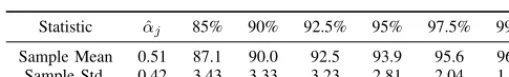
Statistic ↵ˆj 85% 90% 92.5% 95% 97.5% 99% Sample Mean 0.51 87.1 90.0 92.5 93.9 95.6 96.7 Sample Std. 0.42 3.43 3.33 3.23 2.81 2.04 1.63
sample mean of all samples measured in counts per second. ˆ
σD is the sample standard deviation of all samples measured in counts per second.Zˆ↵is an estimate of the standard critical value that will achieve the desired false alarm rate measured in the number of standard deviations above the mean.µˆ↵ is the estimated significance level of threshold Zˆ↵ scaled to FAR measured in alarms per hour. ˆσ↵ is the estimated standard deviation of µˆ↵. ↵ˆl and ↵ˆu are the lower and upper bounds of FAR, respectively, for a 95% confidence interval.
The results of testing each training file with verification data is summarized in Tables III, IV, VI, and VII. Each training data set column number of Table II corresponds to the verification row number result listed in Table III. Each training data set column number of Table V corresponds to the verification row number result listed in Table VI. Measured confidence is in percent and is a function of not only↵ˆl and↵ˆu, but alsoZˆ
↵.
V. CORRECTEDSIGNAL-TO-NOISERATIO
A. Corrected Signal-to-Noise Ratio Definition
1) Signal to Noise Ratio Definition: With a neutron detector setup with ANSI moderation [1], a sample mean of count rate measurements denotedµis acquired using a background
period of 5 minutes. Using a 252Cf source with an emission rate of 20,000 n/s placed at 1.5m from the detector [1], a sample mean of count rate measurements notated⇢is acquired
using a period of 5 minutes. It is assumed in [5][pp.94] that data follow a normal distribution whereσ2
⇡µ. SNR is then defined [5][pp.94] as
SNR, S 2
B =
(⇢−µ)2
µ (15)
2) Sigma Correction Factor: When utilizing a neutron detector to alarm using a specific threshold, the threshold is set using a critical value that assumes that the detector will result in a specific FAR. Section III-C demonstrates how a theoretical standard critical value may result in a measured error rate that is drastically different than the rate that the model predicts.
When comparing two detectors a simple metric often used is SNR. The noise value encompassed by the denominator parameterσrepresents a certain spread of data from the mean that occurs for a specific percent of samples. In other terms, this spread in data can be viewed as occurring at a specific rate for a real-time system. Let’s define a correction factor
γ2 to adjust the measured variance σ2 to account for the disparity between theoretical and measured rates. Using the alarm threshold developed in (3) with the additional correction
factor and notation of this section results in a new alarm threshold
TC=µ+�Z¯↵�
γσ p
NI
(16)
Using the notation of this section and the practical standard critical value of section II-D, the practical threshold results in
TP =µ+
⇣
ˆ
Z↵
⌘ σ
p NI
(17)
To correct the theoretical critical value according to (16) this threshold should be equal to the practical or measured threshold in (17) resulting in
µ+�Z¯↵�pγσ
NI
=µ+⇣Zˆ↵
⌘ σ
p NI
Therefore, if using the theoretical thresholdZ¯↵thenσcould be corrected using the factor
γ= Zˆ¯↵
Z↵
(18)
3) Corrected Signal to Noise Ratio: Using the sigma correction factor in (18) and the approximation σ2 ⇡ µ [5][pp.94], SNR of section V-A1 is adjusted to
SNRγ =
(⇢−µ)2
γ2µ (19)
B. Corrected Signal-to-Noise Ratio Application
1) Backpack Test Overview: With respect to false alarms, the system should tolerate no more than five alarms due to natural background in a 10 hour period [1]. In addition, once the system is configured with an alarm threshold to meet the mentioned error rate, a source that is moving at a specific rate is required to be detected successfully in 96 out of 100 trials [1]. Note that an alarm threshold equal to or greater than the threshold to meet the specified FAR must be used in the moving source test to meet all system requirements.
In the subsequent sections several detector technologies are evaluated using the same parameters. The sampling periods described in section III were used so that the value Z¯↵ = 4.0309results in a false alarm every 2 hours.
2) Fiber Detector Version 1 Test Results: The first fiber detector tested labeled D1 required modification due to an inherent flaw. A standard critical value ofZˆ↵= 5.87resulted in a measured FAR of 0.5 alarms per hour. Using the corre-sponding threshold in a moving source test yielded a detection rate of 90%. Detector D1 measured a background mean of
of background data per scintillating detector for both a6Li op-tical fiber detector and a Li6coated waveguide detector. Using the statistics estimated during training, confidence intervals were constructed at various coefficients and applied across all verification false alarm tests.
In this section several common experimental procedures are followed. Data is acquired with a sample period of 0.2 seconds, an integration period of 4 seconds, and a background period of 5 minutes. Again, the standard critical value is tuned to meet a target FAR of 0.5 alarms per hour.
A. Confidence Interval using Training Data
Each training data set is acquired such that the number of samples ND results in about 70 hours of data to estimate a correctedZˆ↵ in tandem with the FAR performance statistics ˆ
µ↵ andσˆ↵ of section II-C5.
Instead of using the training statistic µˆ↵ over NP B back-ground periods, the target statistic↵ˆjover a single background is used in verification to estimate a confidence interval that models an individual ANSI false alarm experiment [1][pp.17]. The standardized statistic for ↵ˆj is Zj , ↵ˆjσˆ−↵µˆ↵ where the corresponding standard critical value is Z¯↵/2, confidence coefficient is (1 −↵) for ↵ 2 [0,1], and probability of containment is
1−↵=P ✓
−Z¯↵/2< ˆ
↵j−µˆ↵ ˆ
σ↵ < ¯
Z↵/2
◆
(13)
Note that the critical value Z¯↵/2 can be looked up in a standard normal Z table accounting for a two-sided test while
¯
Z↵in (2) uses a single-sided hypothesis test. A realization of a confidence interval [2][pp.216] of FAR for a specific training set is
�
ˆ
↵l,↵ˆu�,�µˆ
↵−�Z¯↵/2�σˆ↵,µˆ↵+�Z¯↵/2�σˆ↵� (14) and is tested for accuracy via the verification data set described next.
B. Containment of Verification Data
Verification data is segmented into background periods and processed like training data as in section II except thatZˆ↵,µˆ↵, andσˆ↵were already calculated via training data. Each verifi-cation data set is acquired such that the number of samplesND results in exactly 10 hours of data. For a given verification data set and j-th background period,↵ˆj is calculated according to (5) usingZˆ↵from training while the selected verification data set is used to calculate both background statistics µˆB,j and ˆ
σj. The value ↵ˆj is tested to determine if contained within the interval in (14). All verification data sets are processed similarly for the j-th background period. In this manner a measured confidence coefficient is calculated as a simple decimal fraction of successful containment. In order to account for background variation, a confidence coefficient is calculated for every possible background period in addition to the j-th and the result is averaged.µ¨↵ is the sample mean and σ¨↵2 is the sample variance of ↵ˆj over every background period and every verification data set.
TABLE II
COATEDDETECTORTRAININGDATASETS
Hours 68.7 71.5 71.8 71.9 71.4 72.4 72.1 95.1
ˆ
µD 0.24 0.22 0.23 0.22 0.23 0.22 0.22 0.24
ˆ
σD 0.25 0.24 0.24 0.24 0.24 0.24 0.24 0.25
ˆ
Z↵ 5.70 5.74 5.83 5.77 5.75 5.68 5.83 5.67
ˆ
µ↵ 0.5 0.49 0.49 0.51 0.51 0.5 0.5 0.5
ˆ
σ↵ 0.58 0.55 0.57 0.62 0.62 0.58 0.54 0.61
ˆ
↵l -0.63 -0.58 -0.62 -0.71 -0.70 -0.64 -0.56 -0.69
ˆ
↵u 1.63 1.56 1.61 1.73 1.72 1.63 1.56 1.69
TABLE III
COATEDDETECTORVERIFICATIONRESULTS FOREACHTRAININGDATA SET
Ver. Sets µ¨↵ σ¨↵ 85% 90% 92.5% 95% 97.5% 99% 128 0.52 0.63 87.6 89.8 91.8 94.0 95.1 96.3 127 0.48 0.60 86.5 89.2 90.2 92.3 94.8 95.8 127 0.40 0.54 92.6 93.6 94.9 95.6 96.4 97.9 127 0.46 0.58 91.8 93.5 94.6 95.5 97.5 98.6 127 0.48 0.61 88.8 92.2 93.0 94.6 95.9 98 127 0.53 0.66 86.7 89.4 91.2 92.5 94.1 96.3 127 0.42 0.56 89.5 91.2 92.8 94.2 96.2 96.8 125 0.54 0.66 86.6 88.4 91.2 92.3 95.8 97.6
TABLE IV
COATEDDETECTORVERIFICATIONRESULTS OVER ALLTRAININGDATA SETS
Statistic ↵ˆj 85% 90% 92.5% 95% 97.5% 99% Sample Mean 0.48 88.8 90.9 92.5 93.9 95.7 97.2 Sample Std. 0.61 3.34 2.90 2.53 2.24 1.90 1.64
TABLE V
FIBERDETECTORTRAININGDATASETS
Hours 67.8 69.7 71.5 71.8 71.9 71.4 72.4 72.1
ˆ
µD 2.28 2.30 2.26 2.28 2.27 2.26 2.25 2.24
ˆ
σD 0.81 0.82 0.81 0.81 0.81 0.81 0.80 0.80
ˆ
Z↵ 4.66 4.80 4.71 4.59 4.66 4.59 4.63 4.58
ˆ
µ↵ 0.5 0.5 0.5 0.5 0.5 0.5 0.5 0.5
ˆ
σ↵ 0.35 0.30 0.31 0.41 0.36 0.44 0.41 0.39
ˆ
↵l -0.18 -0.09 -0.10 -0.30 -0.20 -0.36 -0.30 -0.27
ˆ
↵u 1.18 1.10 1.10 1.29 1.21 1.36 1.30 1.26
TABLE VI
FIBERDETECTORVERIFICATIONRESULTS FOR EACHTRAININGDATA SET
Ver. Sets µ¨↵ σ¨↵ 85% 90% 92.5% 95% 97.5% 99% 125 0.49 0.41 87.6 90.8 92.8 92.8 94.7 96.1 125 0.35 0.30 85.7 85.7 97.0 97.0 97.3 98.1 125 0.44 0.37 84.3 93.3 93.3 95.1 95.1 96.3 125 0.58 0.46 86.5 88.3 91.2 91.2 95.4 96.2 125 0.49 0.40 90.9 90.9 92.7 94.4 96.3 97.2 125 0.59 0.46 88.2 91.6 91.6 93.8 95.5 96.9 125 0.53 0.42 89.0 91.4 93.8 95.6 96.8 97.4 125 0.60 0.47 84.9 87.8 87.8 90.8 93.4 95.9
C. Confidence Testing Results
A total of 8 training files were used per detector with all results listed in each column of Tables II and V. µˆD is the
TABLE VII
FIBERDETECTORVERIFICATIONRESULTS OVERALLTRAININGDATA SETS
Statistic ↵ˆj 85% 90% 92.5% 95% 97.5% 99% Sample Mean 0.51 87.1 90.0 92.5 93.9 95.6 96.7 Sample Std. 0.42 3.43 3.33 3.23 2.81 2.04 1.63
sample mean of all samples measured in counts per second. ˆ
σD is the sample standard deviation of all samples measured in counts per second.Zˆ↵is an estimate of the standard critical value that will achieve the desired false alarm rate measured in the number of standard deviations above the mean. µˆ↵is the estimated significance level of threshold Zˆ↵ scaled to FAR measured in alarms per hour. σˆ↵ is the estimated standard deviation of µˆ↵. ↵ˆl and ↵ˆu are the lower and upper bounds of FAR, respectively, for a 95% confidence interval.
The results of testing each training file with verification data is summarized in Tables III, IV, VI, and VII. Each training data set column number of Table II corresponds to the verification row number result listed in Table III. Each training data set column number of Table V corresponds to the verification row number result listed in Table VI. Measured confidence is in percent and is a function of not only↵ˆland↵ˆu, but alsoZˆ
↵.
V. CORRECTEDSIGNAL-TO-NOISERATIO
A. Corrected Signal-to-Noise Ratio Definition
1) Signal to Noise Ratio Definition: With a neutron detector setup with ANSI moderation [1], a sample mean of count rate measurements denotedµis acquired using a background
period of 5 minutes. Using a 252Cf source with an emission rate of 20,000 n/s placed at 1.5m from the detector [1], a sample mean of count rate measurements notated⇢is acquired
using a period of 5 minutes. It is assumed in [5][pp.94] that data follow a normal distribution whereσ2
⇡µ. SNR is then defined [5][pp.94] as
SNR, S 2
B =
(⇢−µ)2
µ (15)
2) Sigma Correction Factor: When utilizing a neutron detector to alarm using a specific threshold, the threshold is set using a critical value that assumes that the detector will result in a specific FAR. Section III-C demonstrates how a theoretical standard critical value may result in a measured error rate that is drastically different than the rate that the model predicts.
When comparing two detectors a simple metric often used is SNR. The noise value encompassed by the denominator parameterσrepresents a certain spread of data from the mean that occurs for a specific percent of samples. In other terms, this spread in data can be viewed as occurring at a specific rate for a real-time system. Let’s define a correction factor
γ2 to adjust the measured variance σ2 to account for the disparity between theoretical and measured rates. Using the alarm threshold developed in (3) with the additional correction
factor and notation of this section results in a new alarm threshold
TC=µ+�Z¯↵�
γσ p
NI
(16)
Using the notation of this section and the practical standard critical value of section II-D, the practical threshold results in
TP =µ+
⇣
ˆ
Z↵
⌘ σ
p NI
(17)
To correct the theoretical critical value according to (16) this threshold should be equal to the practical or measured threshold in (17) resulting in
µ+�Z¯↵�pγσ
NI
=µ+⇣Zˆ↵
⌘ σ
p NI
Therefore, if using the theoretical thresholdZ¯↵thenσcould be corrected using the factor
γ= Zˆ¯↵
Z↵
(18)
3) Corrected Signal to Noise Ratio: Using the sigma correction factor in (18) and the approximation σ2 ⇡ µ [5][pp.94], SNR of section V-A1 is adjusted to
SNRγ =
(⇢−µ)2
γ2µ (19)
B. Corrected Signal-to-Noise Ratio Application
1) Backpack Test Overview: With respect to false alarms, the system should tolerate no more than five alarms due to natural background in a 10 hour period [1]. In addition, once the system is configured with an alarm threshold to meet the mentioned error rate, a source that is moving at a specific rate is required to be detected successfully in 96 out of 100 trials [1]. Note that an alarm threshold equal to or greater than the threshold to meet the specified FAR must be used in the moving source test to meet all system requirements.
In the subsequent sections several detector technologies are evaluated using the same parameters. The sampling periods described in section III were used so that the value Z¯↵ = 4.0309 results in a false alarm every 2 hours.
2) Fiber Detector Version 1 Test Results: The first fiber detector tested labeled D1 required modification due to an inherent flaw. A standard critical value ofZˆ↵= 5.87resulted in a measured FAR of 0.5 alarms per hour. Using the corre-sponding threshold in a moving source test yielded a detection rate of 90%. Detector D1 measured a background mean of