The Effectiveness of Global Difference Value Prediction And Memory Bus Priority Schemes for Speculative Prefetch

(1)

Abstract

GUNAL, UGUR. The Effectiveness of Global Difference Value Prediction And Memory Bus Priority Schemes for Speculative Prefetch.

(Under the direction of Dr. Thomas M. Conte.)

Processor clock speeds have drastically increased in the recent years. However, the cycle

time improvement in the DRAM semiconductor technology used for memories has been

comparatively slow. The expanding processor – memory gap encourages developers to

find aggressive techniques to reduce the latency of memory accesses.

Value prediction is a powerful approach to break true data dependencies. Prefetching is

another technique, which aims to reduce the processor stall time by bringing data into the

cache before it is accessed by the processor. Recovery-free value prediction [26] scheme

combines these two techniques and uses value prediction only for prefetching so that the

need for validation of predictions and a recovery mechanism for mispredictions are

eliminated.

In this thesis, the effectiveness of using global difference value prediction for

recovery-free speculative execution is studied. A bus model is added for modeling the buses in the

memory system. Three bus priority schemes, First Come First Served (FCFS), Real

Access First Served (RAFS) and Prefetch Access First Served (PAFS), are proposed and

their performance potentials are evaluated when a stride and a hybrid global difference

predictor (hgDiff) is used. The results show that the recovery-free speculative execution

using value prediction is a promising technique that increases the performance

significantly (up to 10%), and this increase depends on the bus priority scheme and the

(2)

THE EFFECTIVENESS OF GLOBAL DIFFERENCE VALUE PREDICTION AND MEMORY BUS PRIORITY SCHEMES FOR SPECULATIVE PREFETCH

by

UGUR GUNAL

A thesis submitted to the Graduate Faculty of North Carolina State University in partial fulfillment of the requirements for

the Degree of Master of Science

COMPUTER ENGINEERING

Raleigh

2003

APPROVED BY:

_________________________________ ________________________________ Dr. Mehmet C. Ozturk Dr. Eric Rotenberg

_______________________________________ Dr. Thomas M. Conte

(3)

Biography

Ugur Gunal was born on April 29, 1980 in Ankara, Turkey. Ugur is the only child of Ipek

and Ibrahim Gunal. Ugur spent 21 years of his life in the Middle East Technical

University campus, where he finished the kindergarten, the primary school, the middle

school and the high school. Ugur spent the majority of these years playing volleyball for

the school team as a captain, going to national and international scout camps and having

soccer games with his friends every week. The international scout camps gave him the

opportunity to see many countries, meet new people and practice his English. After long

and hard years of training, Ugur became a successful scoutmaster. Ugur graduated from

his high school as the first valedictorian in the school’s history. Following his parents’

footsteps, Ugur wanted to continue his education in the Middle East Technical University

and succeeded in his goal. In his senior year, Ugur started working part-time in the VLSI

Design Group of Information Technology & Electronics Research Institute. After being

listed in the High Honor List for 8 semesters and receiving the Highest Departmental

GPA Award for 4 semesters, Ugur graduated with a B.S. degree in Electrical and

Electronics Engineering in June of 2001. Ugur stepped into a new life by leaving his

home and moving to the USA to study at the North Carolina State University to receive

his M.S. degree in Computer Engineering. Ugur worked as a Teaching Assistant for one

year and then joined the TINKER microprocessor design group in May of 2002. Ugur is

currently continuing his research under the supervision of Dr. Tom Conte in the areas of

(4)

Acknowledgements

I would like to dedicate this thesis to my parents; Ipek and Ibrahim, for always supporting

me and making me believe I could succeed in all of my goals. They were always there for

me whenever I needed them, with their endless love and support. They mean much more

than just being my parents; they are also my friends with whom I can share almost

anything. I would like to thank them for being so caring, understanding and wonderful.

I would like to thank my amazing girlfriend Sezen, who filled my life with love, joy and

passion. Together we proved that a long-distance relationship could last, when the love

binding it is strong. From ten thousand miles away, she was still able to charm me with

her unexceptional love and fabulous eyes.

I would also like to thank my grandmother Latife for her loving heart, my uncle Erdo for

being an idol in my life, my aunt Meral for convincing me to make my own decisions and

my grandparents Servin and Osman for all the things they taught me. All of you have

made great contributions to my personality.

In addition, I would like to thank all of my good friends in Turkey, who made my life a

blast. They are very special because they did not let the distance between us ruin our

friendship and I know I can trust all of them in my bad times. In no specific order, I

would like to thank the Sakarya Group (Uygar, Berk, Berkay, and Can), Baris, Cagil,

Meltem, Kerem, Pinar, Doruk, Omer and Yagiz. I could not have asked for better friends.

Thanks also to my scout leaders, Cem and Nihal, and former scouts, Pinar in particular.

I would like especially to thank my committee chair, Dr. Tom Conte, who gave me the

opportunity to work in the TINKER research group. His guidance has helped me to

become a better researcher. I would also like to thank Dr. Eric Rotenberg and Dr.

Mehmet Ozturk for accepting to be my committee members. Thanks also to Nikhil and

members of the TINKER group, Mark and Huiyang. Finally I thank Besiktas, for

(5)

List of Tables

Table 1. Priorities of bus accesses in different priority schemes... 13

Table 2. Cache timings for the block ready and block being loaded cases. ... 16

Table 3. Miss latencies for the memory models. ... 18

Table 4. Base processor configuration. ... 20

(7)

List of Figures

Figure 1. Stride prediction table ... 9

Figure 2. The gDiff predictor... 10

Figure 3. Data cache hit rate... 22

Figure 4. Data cache misses for load instructions... 23

Figure 5. L2 cache hit rate... 24

Figure 6. L2 cache misses for load instructions... 24

Figure 7. Queuing delay for the data cache – L2 cache bus. ... 26

Figure 8. Queuing delay for the L2 cache – memory bus. ... 26

Figure 9. Queuing delay for the instruction cache - L2 cache bus. ... 27

Figure 10. Prediction accuracy and coverage for load instructions. ... 29

Figure 11. Prediction accuracy and coverage for load instructions on the actual path. .... 29

Figure 12. Prediction accuracy and coverage for all value producing instructions. ... 30

Figure 13. Prediction accuracy and coverage for all value producing instructions on the actual path. ... 31

Figure 14. Prediction power of stride and hgDiff predictors... 32

Figure 15. Effect of GVQ Size on Prediction Accuracy and Coverage for the bzip2 Benchmark. ... 33

Figure 16. Effect of GVQ Size on Prediction Accuracy and Coverage for the bzip2 Benchmark. ... 34

(8)

Chapter 1. Introduction and Background

1.1 Overview

Recent advances in microprocessor fabrication technology have drastically increased

processor clock speeds. The cycle time improvement in the DRAM semiconductor

technology used for memories, however, has been slow. As a result, processor – memory

gap continues to grow. This expanding gap encourages developers to find aggressive

techniques to reduce the latency of memory accesses.

The use of a cache is an effective way of hiding memory latency since caches reduce the

number of main memory accesses. However, additional techniques are required to further

reduce the high memory latencies. These include compile-time techniques such as

instruction scheduling, run-time techniques such as non-blocking loads, out-of-order

issue and pre-execution/pre-computation and hardware-based techniques such as write

buffers, victim caches and multi-level caches. Prefetching is one of these techniques,

which aims to reduce the processor stall time by bringing data into the cache or dedicated

prefetch buffers before it is accessed by the processor. An ideal prefetching scheme

would bring the data into the cache just in time for the processor to access it. Accurate

prefetch prediction and sufficient prefetch time are required to improve the overall

system performance.

Data prefetchers can be classified into three categories. Software prefetchers insert

prefetch instructions into the code several cycles before their corresponding memory

instructions so that the requested data can be brought into the cache while the processor

continues computing. They can often take the advantage of compile-time information to

schedule prefetches more accurately than the hardware techniques. However, execution

of the prefetch instructions introduces extra cycles to the processor’s total execution time.

Hardware prefetchers predict future memory-access patterns using the past access and/or

(9)

more memory contention between demand and prefetch requests. Thread-based

prefetchers execute code in another thread context and bring the requested data into the

shared cache before it is accessed by the main thread. They take the advantage of using

the actual code instead of speculating it, which allows them to accurately pre-compute

load addresses. However, the cache misses can prevent the speculative thread from

making faster progress than the main thread and pre-computing the addresses. In this

thesis, a prefetching technique based on speculative pre-execution using value prediction

is studied.

1.2 Previous Work

Several hardware approaches have been proposed for the pre-execution/pre-computation

and prefetching concepts to hide the memory latency.

1.2.1 Prefetching

An early example of prefetching aiming to take advantage of spatial locality is one block

look-ahead (OBL) approach by Smith [24]. In this approach, when block i is referenced,

block i+1 could be prefetched. Depending on when the prefetch is initiated, OBL

implementations differ. In the prefetch-on-miss algorithm, prefetch for block i+1 is

initiated whenever an access for block i misses the cache. In the tagged prefetch

algorithm, each cache block has a tag bit which is set to zero when the block is

prefetched. When the block is fetched and the bit is zero, a prefetch for the next

sequential block is initiated and the bit is set to one.

Chen and Baer [6] introduced a mechanism to predict future data addresses by keeping

track of past data access patterns in a Reference Prediction Table (RPT). RPT is

organized as an instruction cache and each entry in the RPT holds the last address

referenced by that load instruction, the stride (i.e., difference between the last two

(10)

matches an entry in the RPT and the difference between the current address of the load

and the last address stored in the RPT equals the stride, a prefetch for the block at one

offset ahead the current address is initiated. They also proposed a look-ahead scheme by

using a Look-Ahead Program Counter (LA-PC) and a Branch Prediction Table (BPT).

Since LA-PC runs ahead of the normal instruction fetch engine and generates prefetch

requests, they were able to initiate prefetches farther in advance than using the normal

PC.

Reinman et al. [20] examined applying Chen and Baer’s [6] approach to instruction

prefetching. Their architecture uses a single decoupled branch predictor, which can run

ahead of the instruction fetch, instead of two as in Chen and Baer [6]. The branch

predictor produces fetch blocks into a Fetch Target Queue (FTQ), where they are

eventually consumed by the instruction cache. They used the fetch addresses in the FTQ

to perform prefetching for the instruction cache.

Jouppi [15] introduced stream buffers to improve direct mapped cache performance.

Stream buffers are FIFO queues that prefetch successive lines starting at the miss target,

independent of the program context. In order to avoid polluting the cache, lines

prefetched are placed in the buffer and not in the cache. On subsequent misses, the

address of the first item in the stream buffer is compared against the miss address. In case

of a match, cache can be reloaded in a single cycle from the stream buffer.

Palacharla and Kessler [18] enhanced the stream buffers using two techniques: allocation

filters and a non-unit stride detection mechanism. The allocation filter avoids unnecessary

prefetching by allowing a stream buffer to be allocated only after two consecutive misses

for the same stream. For the non-unit stride detection, they dynamically partitioned the

physical address space and detected strided references within each partition. In order to

achieve this they used a history buffer to store currently active partitions and a finite state

machine to detect the stride for references that fall within the same partition. They also

(11)

distance (or delta) between the address of the load and the entries in the history buffer is

found. The delta is then used as a stride for the stream.

Farkas et al. [11] further enhanced stream buffers by using a per-load stride predictor. A

stride is determined for a load instruction by considering only the previous miss

addresses generated by the same load instruction. This differs from the minimum-delta

scheme since the minimum-delta scheme uses global history to calculate the stride for a

given load. They further improved stream buffers by providing them with an associative

lookup capability and a mechanism to avoid the allocation of stream buffers to duplicate

streams.

Sherwood et al. [23] extended the Farkas et al.’s idea [11] for the stream buffers to follow

the correct stream for non-stride based load patterns. They proposed a Predictor-directed

Stream Buffer (PSB) architecture, which uses a predictor to generate an address stream

for prefetching. The predictor is shared among stream buffers and each stream buffer

contains a per-stream history. They used a Stride-Filtered Markov (SFM) predictor.

Correlation-based prefetching is a technique in which a prefetch address is paired with a

current address. A prefetch for an address is initiated when the corresponding block is

referenced or when there is a cache miss to the corresponding block. Pomerene et al. [19]

were the first to apply correlation-based prefetching to data prefetching. They used a

hardware cache to hold the prefetch – current address pair information. Charney and

Reeves [5] extended this mechanism and applied it to the L1 miss reference stream

instead of applying it directly to the load/store stream. They showed that stride based

prefetching could be combined with correlation-based prefetching to give better prefetch

coverage. Joseph and Grunwald [14] used Markov prefetching, which is an evolution of

correlation-based prefetching. They used the miss address stream as their prediction

source and a Markov prediction table to store the addresses that follow a cache miss

address. Each prefetch request has an associated priority and not all prefetch requests

result in a transfer from the L2 cache. They also examined accuracy based adaptivity to

(12)

Shadow Directory Prefetching (SDP), another correlation-based prefetching technique. In

their approach, each L2 cache block contains a second address, i.e. a shadow address.

The shadow address identifies a following address to the corresponding cache block.

When there is a hit in the L2 cache, a prefetch for the shadow address for the

corresponding block is initiated. Alexander and Kedem [1] proposed a mechanism similar

to correlation-based prefetching but used a prediction table distributed over the DRAM

modules. This table is used to prefetch blocks from the large but slow DRAM array into a

small but fast SRAM cache.

Recent prefetching techniques include Content-Directed Data Prefetching by Cooksey et

al. [9], Pointer Cache Assisted Prefetching by Collins et al. [7] and a tag based

prefetching by Hu et al. [13]. Cooksey et al. [9] presented a prefetching scheme without

any history for pointer-intensive applications. In their approach, each address-sized word

of the data is examined for a potential prefetch address. Candidate addresses are

translated and then issued as prefetch requests. As prefetch requests return data from

memory, their contents are also examined for potential prefetch addresses. Collins et al.

[7] introduced a pointer cache, which holds mappings between heap pointers and the

address of the heap object they point to. They examined using the values out of the

pointer cache for value prediction and also initiating prefetching of the first two blocks of

the object pointed-to when a load hits the pointer cache. They further extended the use of

the pointer cache and added it to speculative pre-computation. Hu et al. [13] introduced a

tag-based prefetcher named as Tag Correlating Prefetcher (TCP), which keeps track of

tag sequences per cache-set and the tag correlation patterns. They showed that a small

TCP could outperform a larger address based prefetcher by using the facts that tag

sequences are highly repetitive and easy to predict and a single tag sequence covers

(13)

1.2.2 Pre-execution/Pre-computation

Roth and Sohi [21] proposed speculative data-driven multithreading (DDMT), in which

critical computations are executed in speculative threads called data-driven threads

(DDTs). The DDT fetches and executes only the critical computation and does not

change the architectural state of the machine. They showed that performance can be

improved when computations of loads that are likely to miss in the cache and the

branches that are likely to be mispredicted are executed in DDTs. Collins et al. [8]

extended Roth and Sohi’s idea [21] and explored speculative pre-computation. They

showed that using a basic trigger (i.e., allowing a thread to be spawned only from the

main thread) has two problems. First, if the main thread is stalled, no additional threads

could be spawned. Second, pre-computing the speculative threads many loop iterations

ahead of the main thread is not very effective by this method. In order to overcome these

problems, they proposed chaining triggers, in which a speculative thread can explicitly

spawn another. Zilles and Sohi [28] proposed using speculative slices that execute as

helper threads to avoid cache misses and branch mispredictions for critical instructions.

Their idea is similar to Roth and Sohi’s [21]. However, their control-based scheme

enables the main thread to avoid the latency of re-executing pre-executed instructions by

resolving the mispredicted pre-executed branches at the fetch stage.

Zhou and Conte [26] proposed a recovery-free speculative execution scheme using value

prediction. This is the technique studied in this thesis. Unlike most traditional value

prediction approaches, they focused on using value prediction only for prefetching. A

stride predictor [12, 17, 22] is used to value predict the instructions. At the issue stage, an

instruction is issued un-speculatively if its source operands are ready. However, if they

are not ready and the prediction made in the dispatch stage is confident, then the

instruction is issued speculatively provided that there are enough resources. A

speculatively issued instruction does not leave the issue queue until it is issued

un-speculatively. It writes its result to the physical register file so that its dependent

instructions can be executed speculatively. The speculative result in the register file is

(14)

result is ready and every instruction is executed un-speculatively before it is committed.

Hence, the speculative results do not change the architectural state of the machine.

Therefore, the need for validation of predictions and a recovery mechanism for

mispredictions are eliminated. This is the main difference between their approach and

earlier value prediction schemes.

Pointer chasing, a missing load’s address being dependent on the previous missing load’s

value, is a well-known phenomenon that degrades the performance of a system. In such a

case, if the source operands of the first load instruction are not ready, then both loads will

be stalled in the issue queue if there is no value speculation. The first load will be issued

after its source operands become ready. It will access the cache and will be stalled due to

a cache miss. The second load will be issued only after the first load executes and

produces a value and it will also cause a cache miss. Using the value speculation, the first

load is speculatively issued and causes a cache miss. Prefetching, the process of bringing

the required block into the cache before it is needed, is initiated. This might convert a

cache miss to a cache hit or at least decrease the stall time for the un-speculative

execution of the same load. If the value prediction for the first load instruction is

confident, then the second load instruction uses this value to speculatively execute. The

second load accesses the cache in addition to the first load and starts a prefetch without

waiting for the first load, overlapping the cache misses. In the case of a value

misprediction, the load instruction will miss the cache, just as it would without any

speculation. The disadvantages of value misprediction are cache pollution and increased

memory contention.

The same approach is also used for memory disambiguation. In an un-speculative

machine, load instructions are stalled if there are prior store instructions with unresolved

addresses. Using the technique described above, the loads are issued speculatively for

prefetching as if they were value predicted. They are un-speculatively executed when

(15)

The proposed recovery-free value prediction scheme is similar to the pre-execution

approaches described above. In Zhou and Conte’s approach [26], each confident value

prediction triggers speculative execution of dependent instructions. They execute as a

speculative helper thread to avoid cache misses, even though there is no multi-threading

support. The speculative helper thread is terminated when the un-speculative execution

catches it.

In this thesis, the effect of using a hybrid global difference (hgDiff) value predictor with

Zhou and Conte’s approach [26] is studied. Moreover, to make the memory system more

realistic, a bus model is introduced. The effects of using different priorities for the bus

accesses are also examined.

1.3 Organization of the Thesis

The remainder of the thesis is organized as follows. Chapter 2 explains the stride and

hgDiff predictors used to value speculate instructions. The cache and bus models along

with the bus priority schemes are also discussed in Chapter 2. Chapter 3 explains the

simulation methodology used and presents the results. Chapter 4 concludes the thesis and

(16)

Chapter 2. Architectural Models

2.1 Value Predictors

Value prediction is a powerful technique to break true data dependencies. It can be

performed in two ways, local value prediction and global value prediction. In local value

prediction, the value to be produced by an instruction is predicted by using the values that

are produced by the prior executions of the same instruction. On the other hand, in global

value prediction, the prediction is based on the values produced by all the dynamic

instructions in completion order. Value prediction can also be classified as computational

and context-based. Computational predictors compute some function of the prior values

to make a prediction. The context-based predictors detect a value pattern and predict the

value based on the next value produced when the same pattern repeats.

2.1.1 Stride Predictor

Zhou and Conte [26] used a stride predictor [12, 17, 22] for their recovery-free value

prediction scheme. A stride predictor exploits computational value locality in the local

value history. As shown in Figure 1, it has a PC-indexed table that stores the last value

produced by an instruction and a stride - the difference between the last value and one

before that. Each entry in the table also has a 3-bit confidence counter, which is increased

by 2 when a correct prediction is made and decreased by 1 for a misprediction [25]. The

stride predictor predicts the next value of an instruction by adding the stride to the last

value stored in the prediction table. The prediction is confident if the confidence counter

is greater than 3. The stride predictor is updated speculatively as in [16].

Last value Stride Confidence Counter PC

(17)

2.1.2 Hybrid gDiff Predictor (hgDiff)

In this thesis, the effect of using a hybrid global difference predictor (hgDiff) is studied.

Bodine [2] and Zhou et al. [27] proposed the hgDiff predictor for computational global

value prediction. It is a hybrid of a stride and a gDiff predictor and has the advantage of

exploiting both local and global value localities. A structure called the global value queue

(GVQ) holds the values produced by the selected instructions. These values in the GVQ

are then used to value predict future instructions.

The gDiff predictor has a PC-indexed prediction table that stores the differences between

the value produced by an instruction and the n prior values in the GVQ, as shown in

Figure 2. Each entry in the table also has a selected distance and a 3-bit confidence

counter, which is increased by 2 for a correct prediction and decreased by 1 for a

misprediction [25]. Like the stride predictor, the prediction is confident if the confidence

counter is greater than 3. If the current instruction’s index in the GVQ is x and the

selected distance is y, then the gDiff predictor makes a prediction by adding the value at

entry z in the GVQ to the stored difference diffy, where z=x-y. When a value-producing

instruction completes, the differences between its result and the values stored in the GVQ

are calculated. If any of these differences match the differences stored in the prediction

table for this instruction, then the selected distance is set to the distance for the matching

difference. If there is no match, however, the selected distance is not set and the

differences for this entry are updated with the calculated ones.

Figure 2. The gDiff predictor

valid distance

PC

… _{completing instructions’ results}

prediction

=? =? =? =?

detect match

global value queue prediction update

diff1diff2 … diffk

- - - -

-=?

+

valid distance

PC

… _{completing instructions’ results}

mux

prediction

=? =? =? =?

detect match

global value queue

prediction update

diff diff … dif k

- - - -

-=?

(18)

The stride predictor inserts its predictions into the GVQ at dispatch stage so that they can

be used by the gDiff predictor. Building the GVQ at dispatch time eliminates the pipeline

execution variations due to cache misses and keeps the GVQ ordered. At dispatch stage,

an instruction is value predicted by both stride and gDiff predictors. The gDiff predictor

has a higher priority so if both predictions are confident, the gDiff predictor’s prediction

is used to value speculate the instruction. When a value-producing instruction completes,

it updates both predictors and their confidence counters. The result of the instruction also

updates the GVQ by overwriting the stride prediction for this instruction.

2.2 Cache and Bus Models

The CPU and the memory in a real computer system communicate commonly via a bus.

Contentions on the bus may increase the memory access time and degrade the

performance of the overall system. Since CPU speeds keep increasing at a fast rate and

the performance of many applications is dependent on the observed memory latency, the

buses are playing a greater role in today’s architectures.

Zhou and Conte [26] used a memory hierarchy consisting of an instruction cache, a data

cache and a unified level-2 (L2) cache. In this thesis, a bus model, based on the

Sim-alpha bus model [10], is used to model the buses between the instruction cache and the

L2 cache, the data cache and the L2 cache, and the L2 cache and the memory. The aim is

to use a more realistic memory model and designing these buses to improve the memory

access latency is beyond the scope of this thesis.

There are five different types of accesses to a bus:

A Read Request carries the address of the cache line for which a cache miss occurred. The instruction causing the cache miss must be an un-speculatively

executing load instruction or a store instruction, which is always un-speculatively

(19)

A Read Response is the reply to a Read Request. The requested cache block is sent to the cache, which requested it.

A Prefetch Request is equivalent to a Read Request except the fact that the instruction causing the cache miss must be a speculatively executing load

instruction.

A Prefetch Response is the reply sent to a Prefetch Request, and it is similar to a

Read Response.

A Write Request is sent to the next level in the memory hierarchy when a cache block, that is to be evicted from the cache, is dirty. It carries only the sub-blocks

that are marked dirty, for the corresponding cache block.

There is a separate queue for each bus which holds the accesses that are waiting to be

sent on that bus. These queues are called Bus Queues (BQs). Each access is assigned a

priority according to its type and the bus priority scheme being used. This priority and the

access’ arrival time to a BQ are stored in the corresponding BQ entry. When a bus is idle,

a bus controller selects the next access to be sent on the bus from the candidates in the

corresponding BQ using the stored priorities and the arrival times. The bus controller

selects the candidate with the highest priority. If there is more than one BQ entry with the

highest priority, then the one having an earlier arrival time is selected.

Three bus priority schemes are studied in this thesis. These are First Come First Served

(FCFS), Real Access First Served (RAFS) and Prefetch Access First Served (PAFS).

Table 1 shows the priorities assigned to each type of bus access using these priority

(20)

First Come First

Served

(FCFS)

Real Access First

Served

(RAFS)

Prefetch Access

First Served

(PAFS)

Read Request 0 4 2

Prefetch Request 0 2 4

Read Response 0 5 3

Prefetch Response 0 3 5

Write Request 0 1 1

Table 1. Priorities of bus accesses in different priority schemes.

In FCFS, all of the bus access types have the same priority and the arrival time of a BQ

entry is the only criterion used in the selection of the next bus access. In RAFS, any real

access has a higher priority than a prefetch access, regardless of whether these accesses

are requests or responses. PAFS favors the prefetch accesses over the real accesses, just

as RAFS favors the real accesses over the prefetch accesses. Note that in both schemes, a

Read Response has a higher priority than a Read Request and a Prefetch Response has a

higher priority than a Prefetch Request. This is because the cache miss waiting for a

response occurs earlier than a cache miss producing a request. However, there still exist

certain cases in which a request is more critical than a response for a better performance.

Also, a Write Request has the lowest priority because it does not affect the memory

access time of a load or store instruction. In all of the three bus priority schemes, the

priorities of accesses are constant and do not change with time unless a prefetch access

changes into a real access. How a prefetch access is converted to a real access is

discussed further in this section.

In addition to the buses, sub-blocking and critical word first technique are also added to

the memory model of Zhou and Conte [26]. Bringing a block into a cache by a Read

Response takes several cycles. However, the instruction that caused the cache miss does

not need the whole cache block. Therefore, the cache blocks are divided into sub-blocks.

The instruction can continue execution if the corresponding sub-block is ready even

(21)

instruction can continue executing as the rest of the block is being transferred.

Sub-blocking is also useful in decreasing the size of Write Requests. When sub-Sub-blocking is

used, a write to a sub-block marks it as dirty and when a cache block is evicted from the

cache only the dirty sub-blocks are sent to the next level in the memory hierarchy. When

sub-blocking is not used, however, the whole block has to be sent, which usually wastes

bus bandwidth.

The operation of the caches and the buses can be summarized as follows. The CPU sends

the address of a load/store instruction to the cache. The required block and sub-block are

determined using this address. The cache is checked to see if the corresponding block is

present in the cache.

If the required block is present and ready in the cache, then it is a cache hit and the access time is the hit latency of that cache. The dirty bit of the corresponding

sub-block is set in the case of a store instruction or a writeback.

If the required block is being loaded by a Read/Prefetch Response, then it is checked if the required sub-block has been loaded. If that sub-block is ready, then

it is a cache hit. If not, then the access time is equal to the hit latency of the cache

plus the time it will take for that sub-block to be loaded. If the instruction

accessing the cache is a store, or this is a writeback from the previous level cache,

then the sub-block is marked as dirty.

If the required block is not ready and it is not being loaded, then this is a cache

miss. There are special registers used for cache misses. These are called Miss

Handling Status Registers (MHSRs) and collapse requests for the same cache line.

In addition to storing the address requested from the next level in the memory

hierarchy, each MHSR has an isStore flag which is set to “true” when a store

instruction or a writeback from the previous level requests that address. In order

to distinguish the prefetch accesses from the real ones for accessing the bus, a

(22)

BQ_seqnum is used to locate the bus queue entry holding the bus access for a

miss. isRequired flag is set to “true” if a store or an un-speculatively executing

load is requesting the cache block.

o If the requested address does not match with any of the used MHSR’s address, then it is a non-covered (i.e., new) cache miss and a new MHSR

is allocated. The MHSR’s isRequired flag is set to “true” if this is the data

or instruction cache and the instruction requesting this address is not a

speculatively executing load, or if this is the L2 cache, the access is not a

writeback and the isRequired flag of the corresponding MHSR in the

previous level cache is set. After checking these conditions, if the new

MHSR’s isRequired flag is set to “true”, then a Read Request for the

required block is entered to the bus queue. If it is “false”, then a Prefetch

Request is entered. The bus queue entry number is stored in the MHSR’s

BQ_seqnum field.

o If there is a match between the requested address and an MHSR address, then there is no need to request the same block again. Since the required

cache block has already been requested, the misses are overlapped. This is

called a partially covered miss. If the matching MHSR’s isRequired flag

is not set, then this block has been requested as a prefetch. Just like the

previous case, if this is the data or instruction cache and the instruction

requesting this address is not a speculatively executing load, or if this is

the L2 cache, the access is not a writeback and the isRequired flag of the

corresponding MHSR in the previous level cache is set, then the

isRequired flag of this MHSR must also be set. If the MHSR’s isRequired

flag is changed from “false” to “true”, then the bus queue is checked to see

if there is a corresponding bus queue entry by using the BQ_seqnum field

of the MHSR. There may be a Prefetch Request or a Prefetch Response for

(23)

Response since this block is not only required for a prefetch but also

required for a normal access now. It should be noted that converting a

Prefetch Response to a Read Response is not a realistic approach.

However, this conversion is unlikely to have a great impact on the results.

When a Read/Prefetch Request hits the memory or the L2 cache, or when a block that has

been requested by the data or instruction cache is brought to the L2 cache from the

memory, a Read/Prefetch Response is scheduled. The isRequired flag of the MHSR

waiting for that response determines whether the response is a Read Response or a

Prefetch Response. As explained above, a Prefetch Response can be converted to a Real

Response later while waiting in the bus queue if a non-prefetch access requests the same

block.

Table 2 shows the timings for the memory model used by Zhou and Conte [26] and the

memory model used in this thesis when the required block is ready in the cache, and

when it is being loaded from the next level in the memory hierarchy. The time it will take

for the required block to be loaded is denoted by mhsr.resolved. Similarly,

mhsr.sb_resolved indicates the time it will take for the required sub-block to be loaded.

The hit latency of the cache is denoted by hitLat.

Latency without the bus model Latency with the bus model

Cache block

ready hitLat hitLat

Cache block

being loaded

mhsr.resolved + hitLat

(if mhsr.resolved > hitLat)

mhsr.resolved + 2 * hitLat

(if mhsr.resolved <= hitLat)

mhsr.sb_resolved + hitLat

(if mhsr.sb_resolved > hitLat)

mhsr.sb_resolved + 2 * hitLat

(if mhsr.sb_resolved <= hitLat)

Table 2. Cache timings for the block ready and block being loaded cases.

The bus model introduces extra cycles to Zhou and Conte’s cache timings [26] for the

cache misses. The cache timings for possible cache miss scenarios are presented below.

(24)

hitLat(L1), hitLat(L2), and hitLat(mem) respectively. The L2 cache access time when the

required block is present or being loaded is denoted by accessLat(L2). Note that,

accessLat(L2) represents one of the timings listed in Table 1. For the memory model with

the buses, the data cache – L2 cache bus queuing delay is denoted by qdelay(L1-L2), the

L2 cache – memory bus queuing delay is denoted by qdelay(L2-mem), the latency of

sending a Read/Prefetch Request on a bus is denoted by reqLat, the latency of sending a

Read/Prefetch Response on the data cache – L2 bus is denoted by resLat(L1), the latency

of sending a Read/Prefetch Response on the L2 cache – memory bus is denoted by

resLat(L2), and the time to process returned data and forward it to another bus is denoted

by processLat. The reqLat is a constant since the Read/Prefetch Request size is fixed.

The resLat depends on the cache block size and the bus width. It is calculated using the

formula: resLat = clock differential * (1 + cache block size / bus width), where clock

differential is the ratio of the processor frequency to the bus frequency. The processLat is

1 cycle. While calculating the miss latencies, the latencies and delays are added in the

order of occurrence.

Data cache miss, L2 cache hit:

o Memory model without the buses:

miss latency = hitLat(L1) + accessLat(L2).

o Memory model with the buses:

miss latency = hitLat(L1) + qdelay(L1-L2) + reqLat + accessLat(L2) +

qdelay(L1-L2) + resLat(L1).

Data cache miss, L2 cache miss:

o Memory model without the buses:

(25)

o Memory model with the buses:

miss latency = hitLat(L1) + qdelay(L1-L2) + reqLat + hitLat(L2) +

qdelay(L2-mem) + reqLat + hitLat(mem) +

qdelay(L2-mem) + resLat(L2) + processLat +

qdelay(L1-L2) + resLat(L1).

The bus queuing delays depend on the bus traffic and can vary significantly. Even if all

the buses are idle (i.e., there are no bus queuing delays) when handling a cache miss, the

miss latency for the memory model with the buses is greater than the memory model

without the buses due to the latencies for bus accesses, as shown in Table 3.

Miss latency with the

bus model, when buses

are idle

Miss latency without the

bus model

Additional latencies

introduced by the bus

model

Data cache miss, L2

cache hit

hitLat(L1) + reqLat

+ accessLat(L2)

+ resLat(L1)

hitLat(L1)

+ accessLat(L2) reqLat + resLat(L1)

Data cache miss, L2

cache miss

hitLat(L1) + reqLat

+ hitLat(L2) + reqLat

+ hitLat(mem)

+ resLat(L2)

+ processLat

+ resLat(L1)

hitLat(L1) + hitLat(L2)

+ hitLat(mem)

2 * reqLat + resLat(L2)

+ processLat

+resLat(L1)

Table 3. Miss latencies for the memory models.

(26)

Chapter 3. Experimental Results

In this chapter, the stride and hgDiff predictors are compared and the performance

potential of using different bus priority schemes with these predictors is evaluated.

3.1 Simulation Methodology

The proposed technique is implemented in a cycle-level simulator built using the

SimpleScalar [3] toolset. The underlying processor organization is based on the MIPS

R1000 processor. The base processor configuration is shown in Table 4. The benchmarks

are selected from the SPEC2000 integer benchmark suite. Benchmarks bzip2, gap, gcc

and perl are computation-intensive and benchmarks parser and twolf are

memory-intensive since they have higher data cache miss rates. The reference input data are used

for these benchmarks. The first 800M instructions are fast-forwarded and the next 200M

instructions are simulated. Both predictors have unlimited table sizes, so that they could

be compared without the table size being a limiting factor. The GVQ has 32 entries for

(27)

Instruction Cache Size = 64kB; Associativity = 4-way; Replacement =

LRU; Line Size = 16 instructions (64 bytes); Hit

latency = 1 cycle.

Data Cache Size = 32kB; Associativity = 2-way; Replacement =

LRU; Line Size = 64 bytes; Hit latency = 2 cycles;

32 MHSRs.

Unified Level-2 Cache Size = 512kB; Associativity = 8-way; Replacement

= LRU; Line Size = 128 bytes; Hit latency = 10

cycles; 64 MHSRs.

Memory Hit latency = 80 cycles.

Branch Predictor 64K entry G-share; 32K entry BTB.

Superscalar Core Reorder buffer: 64 entries; Dispatch/issue/retire

bandwidth: 4-way superscalar; 4 fully symmetric

functional units.

Execution Latencies Address generation: 1 cycle; Memory access: 2

cycles (data cache hit); Integer ALU ops: 1 cycle;

Complex ops: MIPS R1000 latencies.

Memory Disambiguation Load stalls when there is a pending store with an

unresolved address.

Value Speculation No value speculation.

Instruction Cache – L2 Cache Bus Bus width = 16 bytes; Clock differential (processor

frequency / bus frequency) = 1.

Data Cache – L2 Cache Bus Bus width = 16 bytes; Clock differential (processor

L2 Cache – Memory Bus Bus width = 16 bytes; Clock differential (processor

Read/Prefetch Request Latency 1 cycle.

Bus Priority Scheme FCFS.

(28)

3.2 Simulation Results

The results using the base processor model are shown in Table 5. In order to evaluate the

effectiveness of the predictors and the bus priority schemes, six different processor

configurations are simulated along with the base model. In the figures, the base model is

labeled as ‘base’ and other configurations are labeled by using the predictor and the bus

priority scheme they use, i.e. the processor using hgDiff predictor for value speculation

and PAFS bus priority scheme is labeled as ‘hgDiff PAFS ’.

Table 5. Baseline results of the benchmarks.

Value speculation is used to break data dependencies so that load instructions that would

otherwise be stalled can be executed speculatively for prefetching the required data for

their un-speculative execution. Hence, this technique should increase the hit rates for the

data cache and the L2 cache. The cache accesses for the prefetches are not counted while

calculating the cache hit rates. The data cache hit rates are shown in Figure 3 and the

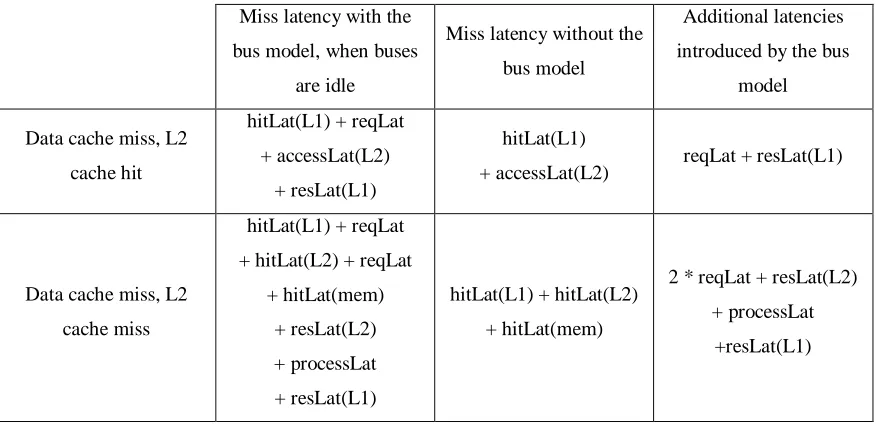
number of data cache misses for load instructions is shown in Figure 4. These cache

misses are divided into non-covered misses and partially covered misses (i.e., the

required block has already been requested from the L2 cache or the memory).

Non-covered cache misses have longer latencies and a greater impact on the overall

performance than the partially covered ones. Figure 3 shows that the proposed technique

increases the data cache hit rate by 1.5% for the memory-intensive benchmarks. For the

computation-intensive benchmarks bzip2, gap and perl the change in the hit rate is

Computation - Intensive Memory- Intensive

bzip2 gap gcc perl parser twolf

IPC 2.02 1.22 1.87 1.28 0.81 0.70

D-Cache Partially covered load misses 494804 38240 873249 375323 3157874 2297266

D-Cache Non-covered load misses 605561 131086 778026 1082292 3124750 4377583

D-Cache Hit Rate (%) 98.22 97.01 94.39 97.98 91.69 89.38

D-Cache - L2 Cache bus queue delay 539105 3897963 10249993 1435030 2974201 16613429

L2 Cache Partially covered load misses 6891 75674 28112 13652 236614 218

L2 Cache Non-covered load misses 98825 87898 85912 112067 1109456 1205872

L2 Cache Hit Rate (%) 84.20 73.09 93.17 93.37 61.64 82.86

(29)

configurations. Figure 4 shows that the proposed technique is effective in reducing the

number of load misses and also increasing the ratio of partially covered misses to overall

misses. This ratio increases because prefetching converts many non-covered load misses

into partially covered ones. The increase in the ratio is around 30% for the bzip2 (27%),

gap (36%), perl (37%) and twolf (33%) benchmarks. The benchmark gcc has the smallest

increase (11%) in the ratio of partially covered loads. Figures 3 and 4 also show that the

data cache hit rate and the ratio of partially covered loads do not depend much on the

predictor or the bus priority scheme being used. The effect of the predictor on the data

cache hit rate is the maximum for the benchmark perl. When the bus priority scheme is

FCFS and a stride predictor is used instead of an hgDiff predictor, the data cache hit rate

increases by 0.6%.

Data Cache Hit Rate

84% 86% 88% 90% 92% 94% 96% 98% 100%

computation-intensive memory-intensive H-Mean

base Stride FCFS Stride RAFS Stride PAFS hgDiff FCFS hgDiff RAFS hgDiff PAFS

(30)

Data Cache Misses for Loads 0 1000000 2000000 3000000 4000000 5000000 6000000 7000000 8000000 bas e S tr id e FC FS S tr ide R A F S Str id e PAF S h g D if f FC FS hgD iff R A F S hgD iff P A F S bas e S tr id e FC FS S tr ide R A F S Str id e PAF S h g D if f FC FS hgD iff R A F S hgD iff P A F S bas e S tr id e FC FS S tr ide R A F S Str id e PAF S h g D if f FC FS hgD iff R A F S hgD iff P A F S bas e S tr id e FC FS S tr ide R A F S Str id e PAF S h g D if f FC FS hgD iff R A F S hgD iff P A F S bas e S tr id e FC FS S tr ide R A F S Str id e PAF S h g D if f FC FS hgD iff R A F S hgD iff P A F S bas e S tr id e FC FS S tr ide R A F S Str id e PAF S h g D if f FC FS hgD iff R A F S hgD iff P A F S

computation-intensive memory-intensive N u m b er o f m isses

Non-covered load misses Partially covered load misses

Figure 4. Data cache misses for load instructions.

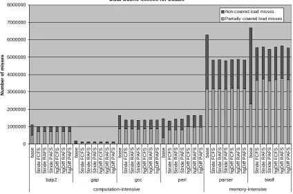
Figures 5 and 6 show L2 cache hit rates and the number of L2 cache misses for load

instructions. It can be seen that the proposed technique does not decrease the L2 cache hit

rate for most benchmarks. Bzip2 and gcc are the two benchmarks for which the L2 cache

hit rate decreases for all used configurations. This greatest decrease is for the bzip2

benchmark (by 2.1%). The increase in the L2 cache hit rate is the maximum for the twolf

benchmark (by 3.3%). Figure 6 shows that the number of load misses is decreased for all

benchmarks and the ratio of partially covered misses is increased for most benchmarks.

The increase in the ratio is the maximum for the gap benchmark (16%). For the

benchmarks gcc, perl, parser and twolf the increase is less than 5% and for the

benchmark bzip2 there is a decrease of 2%. Similar to the data cache, L2 cache hit rate

does not vary much with the predictor type or the bus priority scheme. However, for the

benchmark perl, when the stride predictor is used and the bus priority scheme is changed

(31)

priority scheme is FCFS and an hgDiff predictor is used instead of a stride predictor, the

data cache hit rate increases by 1%.

L2 Cache Hit Rate

0% 10% 20% 30% 40% 50% 60% 70% 80% 90% 100%

computation-intensive memory-intensive H-Mean base Stride FCFS Stride RAFS Stride PAFS hgDiff FCFS hgDiff RAFS hgDiff PAFS

Figure 5. L2 cache hit rate.

L2 Cache Misses for Loads

0 200000 400000 600000 800000 1000000 1200000 1400000 1600000 bas e S tr id e FC FS S tr ide R A F S Str id e PAF S h g D if f FC FS hgD iff R A F S hgD iff P A F S bas e S tr id e FC FS S tr ide R A F S Str id e PAF S h g D if f FC FS hgD iff R A F S hgD iff P A F S bas e S tr id e FC FS S tr ide R A F S Str id e PAF S h g D if f FC FS hgD iff R A F S hgD iff P A F S bas e S tr id e FC FS S tr ide R A F S Str id e PAF S h g D if f FC FS hgD iff R A F S hgD iff P A F S bas e S tr id e FC FS S tr ide R A F S Str id e PAF S h g D if f FC FS hgD iff R A F S hgD iff P A F S bas e S tr id e FC FS S tr ide R A F S Str id e PAF S h g D if f FC FS hgD iff R A F S hgD iff P A F S

computation-intensive memory-intensive N u m b er o f m isses

Non-covered load misses Partially covered load misses

(32)

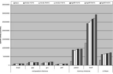
Figures 7 and 8 show the queuing delays on the data cache – L2 cache and the L2 cache –

memory buses. For both buses, using value speculation for prefetching increases the

queuing delay significantly since it increases the number of cache accesses. The increase

in the queuing delay ranges from 6% (Stride FCFS configuration for the benchmark gcc)

to 272% (Stride PAFS configuration for the benchmark gcc) for the data cache – L2

cache bus and from 20% (Stride FCFS configuration for the benchmark perl) to 320%

(hgDiff PAFS configuration for the benchmark parser) for the L2 cache – memory bus.

For the data cache – L2 cache bus, the queuing delay does not vary much with the

predictor type. The average queuing delay for the hgDiff predictor is at most 3% greater

than that of the stride predictor for a selected priority scheme. However, the perl

benchmark is an exception. For this benchmark, the hgDiff predictor has a queuing delay

that is 68% greater than the queuing delay of the stride predictor for the PAFS priority

scheme. Figure 7 also shows that for most benchmarks, the queuing delay is the same for

PAFS and RAFS priority schemes. When compared to the FCFS, the RAFS or PAFS

priority scheme has a greater queuing delay (50% on average) for most benchmarks. The

FCFS has a greater queuing delay than that of the PAFS or RAFS only when a stride

predictor is used for the benchmark perl.

Figure 8 shows that for most benchmarks, the configurations with the hgDiff predictor

have greater queuing delays for the L2 cache – memory bus. Gap is the only benchmark

for which, a configuration with a stride predictor has a greater queuing delay. For the

computation-intensive benchmarks, the queuing delay for RAFS and PAFS priority

schemes are similar and greater than the queuing delay for the FCFS priority scheme (by

21% for the benchmark gcc). For the memory-intensive benchmarks, the PAFS priority

scheme has the longest queuing delay. When an hgDiff predictor is used, the average

queuing delay for the PAFS priority scheme is 8% greater than the average queuing delay

for the FCFS priority scheme. This increase in the average queuing delay is 6% when a

(33)

Data Cache - L2 Cache Bus Queue Delay

0 5000000 10000000 15000000 20000000 25000000 30000000 35000000 40000000 45000000

computation-intensive memory-intensive A-Mean

Q

u

eu

e Del

a

y (

cycl

es)

Figure 7. Queuing delay for the data cache – L2 cache bus.

L2 Cache - Memory Bus Queue Delay

0 5000000 10000000 15000000 20000000 25000000 30000000 35000000

Q

u

eu

e Del

ay (

cycl

es)

(34)

For the benchmark gap, the BQ for the data cache – L2 cache bus holds a maximum of 9

accesses for all used configurations. The BQ for the L2 cache – memory bus holds a

maximum of 8 accesses for the base configuration. This number increases up to 19 for the

stride configurations and up to 18 for the hgDiff RAFS configuration.

Figure 9 shows the queuing delay on the instruction cache – L2 cache bus. It can be seen

that for the benchmarks bzip2, gap, parser and twolf, the instruction cache – L2 cache bus

queuing delay is negligible. For the gcc and perl benchmarks, the queuing delays for

RAFS and PAFS are similar and greater than the queuing delay for the FCFS. When a

stride predictor is used, the queuing delay for the RAFS or PAFS is 1.5 times greater than

the queuing delay for FCFS. The instruction cache – L2 cache bus queuing delay

becomes a limiting factor for the perl benchmark.

Instruction Cache - L2 Cache Bus Queuing Delay

0 100000 200000 300000 400000 500000 600000 700000

Q

u

eu

e

D

e

la

y

(c

ycl

e

s

)

(35)

Figures 10 through 13 compare the accuracies and the coverages of the stride and the

hgDiff predictors for various cases while using the FCFS bus priority scheme. The effect

of the bus priority scheme on the accuracy and coverage of a predictor was observed to

be negligible. This is the reason why the two predictors are compared using only one bus

priority scheme.

Figures 10 and 11 show the accuracies and coverages of the both predictors only for load

instructions. Figure 10 is for all load instructions, whereas Figure 11 is for load

instructions that are on the actual path, i.e. the load instructions that will actually commit

their results. Both figures show that the stride predictor has a better accuracy for most

benchmarks, whereas the hgDiff predictor has a better coverage for all benchmarks. The

difference in the prediction accuracy is the highest for the benchmark gap, for which the

stride predictor has a 6% higher accuracy for all load instructions and a 7% higher

accuracy for load instructions on the actual path. For this benchmark, the hgDiff

predictor’s coverage is around 3.5% greater than that of the stride predictor for both

cases. The difference in the prediction coverage is the highest for the benchmark gcc, for

which the hgDiff predictor has a 6% higher coverage for all load instructions and a 7%

higher coverage for load instructions on the actual path. The stride predictor’s accuracy

for this benchmark is around 3% greater than that of the hgDiff predictor. As an average,

the hgDiff has a 4% higher coverage for all load instructions and the load instructions on

the actual path, whereas the stride predictor has a 2% higher accuracy for all load

(36)

Prediction Accuracy and Coverage for Load Instructions 0% 10% 20% 30% 40% 50% 60% 70% 80% Accu ra cy Cov e rage Accu ra cy Cov e rage Accu ra cy Cov e rage Accu ra cy Cov e rage Accu ra cy Cov e rage Accu ra cy Cov e rage Accu ra cy Cov e rage

computation-intensive memory-intensive A_mean

Stride FCFS hgDiff FCFS

Figure 10. Prediction accuracy and coverage for load instructions. Prediction Accuracy and Coverage for Load Instructions on the Actual Path

0% 10% 20% 30% 40% 50% 60% 70% 80% 90% 100% Accu ra cy Cov e rage Accu ra cy Cov e rage Accu ra cy Cov e rage Accu ra cy Cov e rage Accu ra cy Cov e rage Accu ra cy Cov e rage Accu ra cy Cov e rage

(37)

Figures 12 and 13 show the accuracies and coverages of the both predictors for value

producing instructions. Figure 12 is for all value producing instructions, whereas Figure

13 is for those instructions that are on the actual path. The results for all value producing

instructions are similar to the results for the load instructions. The hgDiff predictor has

better coverage for all benchmarks, whereas the stride predictor has better accuracy for

all benchmarks except the twolf benchmark. For this benchmark, the hgDiff predictor

accuracy is 2% greater than the stride predictor accuracy and the hgDiff predictor

coverage is more than 3% greater than the stride predictor coverage regardless of whether

the value producing instructions are on the actual path or not. The coverage of the hgDiff

predictor is 5% greater than that of the stride predictor for the benchmark gcc and the

accuracy of the stride predictor is more than 2% greater than that of the hgDiff predictor

for the benchmarks gcc and perl.

Prediction Accuracy and Coverage for All Instructions

0% 10% 20% 30% 40% 50% 60% 70% 80% 90% Accu ra cy Cov e rage Accu ra cy Cov e rage Accu ra cy Cov e rage Accu ra cy Cov e rage Accu ra cy Cov e rage Accu ra cy Cov e rage Accu ra cy Cov e rage

(38)

Prediction Accuracy and Coverage of All Instructions on the Actual Path 0% 10% 20% 30% 40% 50% 60% 70% 80% 90% 100% Accu ra cy Cov e rage Accu ra cy Cov e rage Accu ra cy Cov e rage Accu ra cy Cov e rage Accu ra cy Cov e rage Accu ra cy Cov e rage Accu ra cy Cov e rage

Figure 13. Prediction accuracy and coverage for all value producing instructions on the actual path.

Bodine [2] used the prediction power to compare predictors with varying strengths in

accuracy and coverage. The prediction power is defined as the product of the accuracy

and coverage of the predictor. Figure 14 shows the prediction powers of the stride and

hgDiff predictors. Each predictor’s prediction power is calculated for load instructions

and for all value producing instructions. The hgDiff predictor has a prediction power,

which is 0.5% (for the benchmark perl) to 2.2% (for the benchmark bzip2) greater than

the stride predictor for load instructions. The hgDiff predictor is superior to the stride

predictor also for all value producing instructions, except for the bzip2 benchmark. As an

average, the hgDiff prediction power is greater than the stride prediction power by 1.3%

(39)

Prediction Power

0% 5% 10% 15% 20% 25% 30% 35% 40% 45% 50%

Loads All Loads All Loads All Loads All Loads All Loads All Loads All

Figure 14. Prediction power of stride and hgDiff predictors.

Previous studies [2, 27] show that the hgDiff predictor has greater prediction coverage

than the stride predictor. They also show that the prediction accuracy of the hgDiff

predictor is greater than that of the stride predictor on average. However, this contradicts

with the results presented in this thesis. The reason for this discrepancy is the speculative

update used for the stride predictor. The speculative update increases the performance of

the stride predictor significantly. Since the correct stride predictions entered into the

GVQ increase the accuracy of the gDiff predictor, speculative update also increases the

performance of the gDiff predictor. However, this increase is not as significant as the

increase in the stride predictor’s performance because the GVQ size starts to become a

bottleneck for the gDiff predictor. If an instruction has a stride pattern and the execution

of the instruction is completed before it is dispatched again, then the speculative update is

not used and both predictors can predict this instruction correctly. Then, if the same

instruction is dispatched multiple times before the current execution of that instruction is

(40)

the GVQ size is small, the result from the prior execution of the same instruction gets

overwritten by another instruction’s result and when the current execution of this

instruction is completed, the correct difference cannot be calculated. Therefore, the gDiff

predictor starts making incorrect predictions, whereas the stride predictor keeps correctly

predicting the instruction since it does not depend on the GVQ size.

The effects of the GVQ size on the hgDiff prediction accuracy and coverage can be seen

in Figures 15 and 16. Figure 15 shows that for the bzip2 benchmark, the hgDiff

prediction coverage increases as the GVQ size increases. The accuracy is not affected

significantly; however, it decreases when the GVQ size is increased beyond 64. Figure 16

shows that for the benchmark gap, changing the GVQ size from 16 to 32 increases the

hgDiff prediction accuracy and coverage significantly. When the GVQ size is increased

to 64, the hgDiff prediction accuracy becomes greater than the stride prediction accuracy.

Further increasing the GVQ size does not provide much benefit for the gap benchmark.

Effect of GVQ Size on Prediction Accuracy and Coverage for the bzip2 Benchmark

50% 55% 60% 65% 70% 75% 80% 85%

GVQ size = 16 GVQ size = 32 GVQ size = 64 GVQ size = 128 GVQ size = 256

Stride hgDiff hgDiff hgDiff hgDiff hgDiff

Accuracy (All) Coverage (All)

(41)

Effect of GVQ Size on Prediction Accuracy and Coverage for the gap Benchmark

25% 35% 45% 55% 65% 75% 85%

GVQ size = 16 GVQ size = 32 GVQ size = 64 GVQ size = 128 GVQ size = 256

Stride hgDiff hgDiff hgDiff hgDiff hgDiff

Accuracy (All) Coverage (All)

Figure 16. Effect of GVQ Size on Prediction Accuracy and Coverage for the bzip2 Benchmark.

Figure 17 shows the speedups of the proposed speculative execution technique using six

different configurations. Although the hgDiff predictor has a better prediction power, the

speedups of the configurations with the hgDiff predictor are smaller than the speedups of

the configurations with the stride predictor for all benchmarks except the gap benchmark.

For this benchmark, both predictors have the same prediction accuracy, but the hgDiff

predictor has a better coverage. Also, the L2 cache – memory bus queuing delay is less

for the configurations with the hgDiff predictor. For the benchmarks bzip2 and perl, the

speedups of the configurations with hgDiff predictor are negative. For the benchmark

bzip2, using an hgDiff predictor results in a decreased L2 cache hit rate and an increased

L2 cache – memory bus queuing delay. For the benchmark perl, the queuing delays for

both data cache – L2 cache and L2 cache – memory buses increase when an hgDiff

(42)

For a given benchmark, the effect of the bus priority scheme is usually the same for both

predictors. When using the hgDiff predictor, the RAFS priority scheme provides the

greatest speedups for all benchmarks except the twolf benchmark, for which the PAFS

priority scheme outperforms the other priority schemes. When using the stride predictor,

the RAFS priority scheme provides the greatest speedups for the bzip2, gap, gcc and

parser benchmarks. The PAFS priority scheme provides the smallest speedups for the

bzip2, gap, perl and parser benchmarks. However, it outperforms the other priority

schemes for the twolf benchmark. The greatest impact of the bus priority scheme on the

speedups is observed for the perl benchmark when using a stride predictor. For this case,

the FCFS priority scheme provides a speedup that is almost 4 times greater than the

speedup provided by the other two priority schemes. The FCFS priority scheme provides

greater speedup than the RAFS and PAFS priority schemes because the instruction cache

– L2 cache queuing delays for these two schemes are much greater than the queuing

delay for the FCFS priority scheme.

Speedups

-2% 0% 2% 4% 6% 8% 10% 12%

computation-intensive memory-intensive H-Mean

Stride FCFS Stride RAFS Stride PAFS hgDiff FCFS hgDiff RAFS hgDiff PAFS

(43)

The results show that using the recovery-free speculative execution, the performance is

increased significantly, especially for the memory-intensive benchmarks. Using the stride

predictor provides more benefit over the hgDiff predictor for most benchmarks. The bus

priority schemes affect the overall performance. The RAFS priority scheme provides

better speedups for most benchmarks for both predictors. When compared to Zhou and

Conte’s results [26], the proposed recovery-free speculative execution technique with a

more realistic memory model provides greater speedups especially for the perl and the

memory-intensive benchmarks. The main reason for this is that the base model presented

in this thesis usually has a lower IPC than the base model used by Zhou and Conte [26]

for a given benchmark due to the contentions on the buses. Another reason could be the

unlimited table size of the stride predictor used in this thesis, as opposed to the 4K entry

The Effectiveness of Global Difference Value Prediction And Memory Bus Priority Schemes for Speculative Prefetch

Biography

Acknowledgements

Contents

List of Tables

List of Figures

Chapter 1.

Introduction and Background

Chapter 2.

Architectural Models

Chapter 3.

Experimental Results