ABSTRACT
LANDGE, SWAPNIL JAYANT. Employing Simulation Modeling in the Lean Six Sigma Methodology. (Under the direction of Dr. Jeffrey Joines and Dr. Stephen Roberts).
Lean and Six Sigma concepts have brought tremendous change in the world. The notion of removing wastes using the Lean tools from a system coupled with the statistical data analysis of Six Sigma embedded into a continuous improvement framework has become standard practice in process improvement in a variety of manufacturing industries, health care and other service systems, and business offices. In certain cases, the implementation of change may face government red tape, permissions, financial hurdles and time constraints. Most Lean Six Sigma projects fail at the improvement stage or control stage either due to barriers of cost, time or permission to implement the change. They might fail because the improvements implemented were costly but did not realize enough gains.
Employing Simulation Modeling In the Lean Six Sigma Methodology
by
Swapnil Jayant Landge
A thesis submitted to the Graduate Faculty of North Carolina State University
in partial fulfillment of the requirements for the degree of
Master of Science
Industrial Engineering and Textile Engineering (Co-Major)
Raleigh, North Carolina 2015
APPROVED BY:
_______________________________ ______________________________ Dr. Jeffrey Joines Dr. Stephan Roberts
Committee Co-Chair Committee Co-Chair
________________________________ ________________________________ Dr. Russell King Dr. Jerome Lavelle
iii BIOGRAPHY
Swapnil J. Landge was born on July 20, 1990, in the city of Vadodara, India to Jayant Landge and Kalika Landge. In June 2008, he completed graduated from Don Bosco High School in Vadodara. In June 2012 finished his Bachelor’s Degree with First Class in Textile Engineering from The Maharaja Sayajirao University of Baroda. He is very interested in product development and entrepreneurial activities. He has also been actively involved in organizing national-level technical and non-technical events for his college as well as campus recruitment events. During his undergraduate education, he started building websites for corporate and academic institutions as a hobby. After graduation, he invented a device for measuring yarn length and registered a patent. Based on his invention, he developed a product-based enterprise called “textil inc.” and started selling this product to some of the textile industries. In early 2013, he registered a second patent on his spiral coiling machine for Card and Draw-frame machines. During the summer of 2014, he designed an electromagnetic water pump called i-jet for nail salons and this product is going to be commercialized in July 2015.
iv ACKNOWLEDGMENTS
The author would like to thank Dr. Joines for his tireless efforts and guidance throughout the project. He would like to heartily thank him for the knowledge he shared with the author and helped him understand some of his weaknesses and strengths. The author greatly respects him for his patience and his principles. Moreover, he would also like to thank Dr. Roberts for his guidance on the project and thesis. His expertise and detailed thinking ability inspired the author to understand the level of thinking one should cultivate while approaching a project.
v TABLE OF CONTENTS
LIST OF TABLES………....…....viii
LIST OF FIGURES………..…...…...ix
Chapter 1
Introduction
... 1Chapter 2
Literature Review
... 42.1Six Sigma and Design for Six Sigma ...4
2.1.1 DMAIC Process ... 6
2.2 DMADV Process ...10
2.2.2 DFSS vs DMAIC ... 12
2.3 Lean Systems ...12
2.4 Simulation ...17
2.4.1 Simulation Types ... 18
2.4.2 Simulation Methodology ... 20
2.5.1 Simulation in Six Sigma and Design for Six Sigma ... 23
2.5.2 Simulation in Lean ... 26
Chapter 3
Research Methodology
... 283.1Define Phase ...28
3.1.1 Mapping the Process ... 30
3.1.2 Understanding Worker Behavior ... 34
3.2Measure Phase ...35
3.2.1 Data Collection at the DMV ... 36
3.2.2 Issues with the Data ... 40
3.2.3 Input Modeling ... 42
3.3Analyze Phase ...45
3.3.1 Building the Initial Current State Simulation Model of the DMV ... 47
vi
3.3.3 Validation and Verification of the Model ... 68
Chapter 4
Data Analysis and Results
... 734.1 Improve Phase ...73
4.1.1 Looking at 7:00 AM Start ... 74
4.1.2 Optimizing the Starting Times for Additional Workers ... 81
4.1.3 Optimizing Three Additional Workers ... 82
4.1.4 Optimizing Two Addional Workers ... 88
4.1.5 Adding One Additional Worker ... 90
4.1.6 Comparing Best Starting Schedules for Different Number of Workers . 92 4.1.7 Effect of Adding Three Temporary Workers ... 102
4.2Control Phase ...109
Chapter 5
Conclusions and Future Work
... 1115.1Summary of Conclusions ...111
5.2Limitations and Recommendations ...112
5.3Future Work ...113
References ... 115
Appendices ... 118
vii LIST OF TABLES
Table 2.1: DMAIC Process...6
Table 2.2: DMADV Process ...11
Table 2.3: Seven Wastes of Lean Principles ...13
Table 3.1: Distributions that Were Used to Model the DMV ...45
Table 3.2: Fields of the Customer Table ...50
Table 3.3: Customer Processing Time Table ...52
Table 3.4: Added State Variables and Properties of the Worker Object ...54
Table 3.5: Added State Variables of the ModelEntity ...60
Table 4.1: Scenarios of Different Schedules for 14 Workers (Three Additional Workers) and its Effect on Time in System (Monday) ...85
viii LIST OF FIGURES
Figure 2.1: Lean Guiding Principles ...15
Figure 2.2: Graphical Representation of 24 Lean Tools and Their Broader Categories (taken from Goforth, 2007) ...16
Figure 2.3: Lean Six Sigma DMAIC Process Overview with Tools ...17
Figure 2.4: Simulation Model of a Process ...18
Figure 3.1 DMV office Process flow chart ...32
Figure 3.2: Flow chart for customers taking a road test ...32
Figure 3.3: Flow Chart for Customers Taking Written Test...33
Figure 3.4: Flow chart for customers needing a State ID card, reinstatement or other transactions ...34
Figure 3.5: Understanding the system behavior based on the location ...34
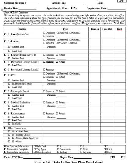
Figure 3.6: Data Collection Plan Worksheet ...38
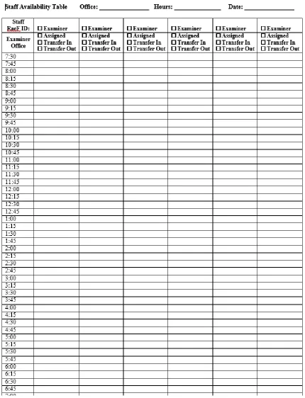
Figure 3.7: Examiner Availability Data Collection Plan ...39
Figure 3.8: Problems with some of the collected data and how simulation served useful in finding solution to the problems ...41
Figure 3.9: Fitted Distribution for Other Transaction Customer Type ...44
Figure 3.10: Portion of the SIMIO™ Customer Data Table ...51
Figure 3.11: Customer Processing Time and Priority Table ...53
ix
Figure 3.14: Process Executed When each Worker is Created ...56
Figure 3.15: Worker Schedule Table ...57
Figure 3.16: Process used to update the Capacities of the Workers for Every Time Interval of the Worker Schedule Table ...57
Figure 3.17: Waiting for the Number in System to go to Zero After 5:00 PM ...58
Figure 3.18: Specifying the SetServerAvailability Process on the Entering and Exiting of a Node ...59
Figure 3.19: Set Server Availability Generic Process ...59
Figure 3.20: Process to Reject Customer’s Request ...62
Figure 3.21: Generic Process Logic for Customers Entering/Exiting Workstation ..63
Figure 3.22: Customer Reaches the Outside for the Road Test ...65
Figure 3.23: Changing the Picture to look like a Car ...65
Figure 3.24: Customer and Evaluator Arrive Back to Office ...66
Figure 3.25: Balking Logic Process Diagram ...66
Figure 3.26: System Break Down Process and Removal ...67
Figure 3.27: Remove all Customers Waiting for a Road Test ...68
Figure 3.28: Sensitivity of Different Input Parameters on the Output ...70
Figure 3.29: Confidence Interval of Simulated Data ...71
Figure 3.30: Animated Model of Charlotte DMV Office ...72
Figure 4.1: Effect of the Number of Workers on the Average Time in System ...75
x Figure 4.3: Comparison of Old and New System by Changing Number of Workers and
its Effects on the Average Time Spent in Waiting Queue ...77 Figure 4.4: Number of Balking Customer Comparison between Old and New Systems
...78 Figure 4.5: Comparison of Number of Customers Seen between Old and New Systems
...79 Figure 4.6: Average Time in System for Each Day of the Week of High and Low
Volume Month ...80 Figure 4.7: Comparison of Average Time in System between Low-Volume and
High-Volume Month by Day...80 Figure 4.8: Worker Notation Explanation...81 Figure 4.9: Time in System Based on Hour with Best Scenarios Selected Using KN
Algorithm for 14 Workers with Different Starting Times for a Monday of Mid-Volume Month ...83 Figure 4.10: Average Time in System Based on Hour with Best Scenarios Selected using
KN Algorithm for 14 Workers with Different Starting Times for a Monday of High-Volume Month ...84 Figure 4.11: Scenarios of Different Schedules for 14 Workers (Three Additional
Workers) and its Effect on Average Time in System (Monday) ...85 Figure 4.12: Scenarios of Different Schedules for 14 Workers (three additional workers)
xi Figure 4.13: Scenarios of Different Schedules for 14 Workers (three additional workers)
and its Effect on Average Time in System (Friday) ...87 Figure 4.14: Scenarios of Different Schedules for 14 Workers (three additional workers)
and its Effect on Number of Balkers (Friday) ...88 Figure 4.15: Scenarios of Different Schedules for 13 Workers (two additional workers)
and its Effect on Average Time in System (Monday) ...89 Figure 4.16: Scenarios of Different Schedules for 13 Workers (two additional workers)
and its Effect on Average Time in System (Friday) ...90 Figure 4.17: Scenarios of Different Schedules for 12 Workers (one additional worker)
and its Effect on Average Time in System ...91 Figure 4.18: Scenarios of Different Schedules for 12 Workers (one additional worker)
and its Effect on Time in System(Friday) ...92 Figure 4.19: KN Algorithm-based Best Scenarios of Different Worker Populations and
their Effect on Average Time in System (Monday, Mid-Volume)...93 Figure 4.20: Time in System over the Time Customer Arrives ...93 Figure 4.21: KN Algorithm-based Best Scenarios of Different Worker Populations and
their Effect on Average Time in System (Monday, High-Volume) ...94 Figure 4.22: KN Algorithm-based Best Scenarios of Different Worker Populations and
their Effect on Average Time in System (Friday, Mid-Volume) ...95 Figure 4.23: Number of Balking Customers for a Monday of Mid-Volume Month based
xii Figure 4.24: Number of Balking Customers for a Friday of High-Volume Month based
on the Number of Workers Present ...97 Figure 4.25: KN Algorithm-based Best Scenarios of Different Worker Populations and
their Effect on Time in System (Friday, High -Volume) ...98 Figure 4.26: Number of Customers Served on Monday of a Low-Volume Month with
Different Numbers of Workers and Best Schedules Selected Based on KN Algorithm ...99 Figure 4.27: Number of Customers Served on Monday of a Mid-Volume month with
Different Numbers of Workers and Best Schedules Selected Based on KN Algorithm ...99 Figure 4.28: Number of Customers Served on Monday of a High-Volume month with
Different Numbers of Workers and Best Schedules Selected Based on KN Algorithm ...100 Figure 4.29: Number of Customers Served on Friday of a Low-Volume Month with
Different Numbers of Workers and Best Schedules Selected Based on KN Algorithm ...101 Figure 4.30: Number of Customers Served on Friday of a Mid-Volume Month with
Different Numbers of Workers and Best Schedules Selected Based on KN Algorithm ...101 Figure 4.31: Number of Customers Served on Friday of a High-Volume Month with
xiii Figure 4.32: Effect of Temporary Workers Working from 7 AM to 11 AM on Average
Time in System per hour ...103
Figure 4.33: Effect of Temporary Workers Working from 10 AM to 2 AM on Average Time in System per hour ...104
Figure 4.34: Average Time in System for Different Full and Part Schedules ...106
Figure 4.35: Comparing Different Part Time Schedules for One, Two and Three Temps ...107
Figure 4.36: Effect of Temporary Workers Working from 7 AM to 11 AM on the Number of Balking Customers ...108
Figure 4.37: Effect of Temporary Workers Working Full and Part Time on the Number of Customers Served ...109
Figure 72: Greensboro Office Model ...119
Figure 73: Durham Office Model ...120
1
Chapter 1
Introduction
Since the time they have existed, people have been trying to improve them in order to reduce cost and raise productivity because the profit margins are very low. This has been especially true for manufacturing systems. Henry Ford simplified and optimized the assembly line for making cars by reducing setups and producing cars more quickly. These process improvements led to producing cars that were less costly and thus more affordable for consumers. These same concepts were introduced in the 19th century in meat packing and textile mills. Ad hoc methods of process improvement have been used for quite some time. After World War II, Japanese companies were facing a resource crisis; hence, the Lean manufacturing concept started as a way to systematically eliminate wastes such as over-production or defects in any system in order for businesses to survive. Implementing Lean as a continuous improvement philosophy helped the Japanese auto companies who owned very little world market share to become the world leader. Lean thinking was born there and brought back to the US in later years.
2 what others had been doing using statistical quality data and placed it inside of a continuous improvement framework called Six Sigma where the five stages were define, measure, analyze, improve, and control (DMAIC). Others like Jack Welch of GE took Six Sigma beyond manufacturing and applied it to improve all aspects of the corporation. In many cases, the tools that were already available were packaged into a framework that was consistent every time the methodology was applied.
Since its creation, people have been using the computer to be build virtual systems of the real world. In the late 1980s, as computer systems became more accessible and faster, people began building simulation models of manufacturing as well as service systems to analyze them. These virtual systems allowed the designers to play “what if” scenarios to make improvements or make better decisions without costly mistakes or interacting with the real system. Simulation Modeling tools have gained wide acceptance across many different industries. In recent years, the tools of Lean have been embedded into the Six Sigma process to produce the Lean Six Sigma methodology. While a simulation tool is an improvement methodology and can act as another tool during the methodology, it has not been widely used during Lean Six Sigma projects.
3 simulation modeling offers a potential tool to carry out all possible changes and improvements in a virtual environment which may be more cost effective and quicker.
4
Chapter 2
Literature Review
As mentioned previously, Lean thinking, Six Sigma, and Simulation Modeling are all tools used in improvement of processes. Most process improvement methodologies deal with systems that are complex and rarely perform the way they are expected to. These three tools are often used in combination with one another as will be described.
2.1 Six Sigma and Design for Six Sigma
5 Six Sigma evolved from other quality initiatives such as International Organization for Standardization ISO, Total Quantity Management (TQM) and Baldrige to become a quality standardization process based on hard data and not hunches or gut feelings, hence the mathematical term, Six Sigma. Six Sigma utilizes a host of traditional statistical tools but encompasses them within a process improvement framework. These tools include affinity diagrams, cause & effects, failure modes and effective analysis (FMEA), Poka Yoke (mistake proofing), survey analysis (voice of customer), design of experiments (DOE), capability analysis, measurement system analysis, statistical process control charts and plans, etc. (Lee and Choi, 2006; Mellat-Parast and Digman 2011; Hilton and Sohal, 2012).
6 phase is reached. The stages often feedback to previous stages as data is gathered and analyzed.
2.1.1 DMAIC Process
The Six Sigma method is based on the DMAIC process and is utilized when the product or process already exists but it is not meeting the specifications or performing adequately as described in Table 2.1. Several different tools are used throughout the methodology.
Table 2.1: DMAIC Process
Step Description
Define Identify, prioritize and select the right projects. Once determined, then define the project goals and deliverables for the problem.
Measure Define the key product/process characteristics to create a baseline by gathering data.
Analyze Identify the key process determinants and/or root causes of variability. Improve Develop solutions and optimize performance by eliminating defects.
Control Sustain the current gains and future process performances.
2.1.1.1 DMAIC – Define
7 Voice of the customer (VOC) data is used to establish the CTQs. The Supplier, Inputs, Process, Outputs and Customers (SIPOC) is a high-level diagram to identify who are the external and internal suppliers and customers, determine the inputs and outputs to the process, and develop a 10,000 foot view of the process (i.e., five or seven process steps). SIPOC can assist in identifying the root cause analysis, and data that need to be collected, including VOC data from all customers. A detailed process map can be used to fully understand the entire process by identifying potential failures, data collection points, boundaries, etc. (Breyfogle, 2003).
2.1.1.2 DMAIC – Measure
The measure phase is the next step where sample data is gathered to be considered for analysis and the establishment of baseline to determine if improvement has occurred. Metrics are established to that will measure/determine if CTQs are met. Many tools can be used to establish a baseline (i.e., capability analysis, Pareto or run charts). If customer specifications are present (i.e., lower (LSL) and/or upper (USL) specification limits) capability analysis can be calculated which can determine capability of the current process. The terms Cp and Cpk are calculated using the upper and lower specifications, the mean of the process data (x) and the standard deviation of the data (sˆ ). Cp measures if the process is capable of meeting the
8 ˆ * 6 ) LSL U ( ) ( s SL Cp best
ˆ * 3 ) LSL x , x U ( s SL Min Cpk
In this phase, a thorough brainstorming is done to identify the project metrics and potential root causes and determine the necessary data requirements to gauge the project deliverables. During this phase, careful consideration of whether data is to be collected once or several times is necessary, recognizing the difficulties in repeating the data collection. Some of the useful tools used for this step are a data collection plan and measurement system analysis (MSA). The data collection plan is the developed method or the tables that are to be used to collect the data and is very important when the Six Sigma team may not be the ones actually collecting the data. The Six Sigma team decides what should be recorded and the frequencies and accuracy of the data collected. Measurement systems analysis determines the capability of the system used to measure. This analysis shows how repeatable and reproducible the measurement system is (i.e., how much variation is due to the process versus the system used to collect the data).
2.1.1.3 DMAIC – Analyze
9 perform hypothesis testing and establish relationships between independent and dependent variables using regression and correlation. Histograms are used to check the nature and distribution of the data while Pareto charts are used to identify the severity (i.e., frequency) of causing factors. Fish bone or Ishikawa diagrams are used to analyze the cause and effects of the variation in the response metrics. Failure mode effects analysis (FMEA) is used to identify the modes of failures and their effects. Each mode of failure is given severity level, probability of occurrence and risk level, which are computed based on the level of severity based on frequency of occurrence. These modes are often identified from the SIPOC or process maps from the define stage. The 5 whys are used to question why is something occurring to get to the root cause. The analysis step is used to determine the baseline as well as what x’s are potentially causing the variation in the system.
2.1.1.4 DMAIC – Improve
10 to some of the new design methodologies since this method does not take account potential interactions among the independent variables. There are several DOE designs (i.e., full and fractional factorial, response surface, etc.) used to screen out factors of importance to determine a relationship among the dependent and independent variables. Multiple runs (i.e., replicates) may be necessary to determine which causes are the most important and the best values for these inputs. It is very important once solutions to the problem are found that a pilot is run to determine the true effect of the change.
2.1.1.5 DMAIC – Control
The objective of this phase is to sustain the improvements yielded during the improvement stage through a control plan. The control plan uses statistical control charts for monitoring, training workers, and visual controls to determine a problem before it happens.
2.2 DMADV Process
11 Table 2.2: DMADV Process
Step Description
Define Determine customer needs and specifications through voice of customer and then identify metrics to meet the CTQs.
Measure Based on the objectives set during define phase, Measure the required inputs for analysis.
Analyze Identify the key process options necessary to meet the customer needs. Design Design a detailed process or product that will meet the customer needs as
well as be a Six Sigma product/process.
Verify Make sure the design performance and ability will meet the customer needs where the customer can be internal and/or external to the organization.
2.2.1.1 DMADV – Design
The first three phases of the DMADV process are similar to the DMAIC method except one relies heavily on VOC, both internal and external to the process, to really determine the customer needs and establish metrics to measure those needs which will be used in the design phase to evaluate design alternatives. Unlike DMAIC, the fourth step is development of the new process or product. The process or product is designed from the start to meet Six Sigma standards, and hence it is technically termed as DFSS (Design for Six Sigma). The main objective of the design phase is to design the process or product according to the customer needs using the house of quality (i.e., quality function deployment (QFD)), benchmarking, prototyping, and robust selection (Breyfogle, 2003)
2.2.1.2 DMADV – Verify
12 verify phase is to ensure that the product or process will follow a Six Sigma quality standard when delivered to the internal or external customer.
2.2.2 DFSS vs DMAIC
There are several times throughout a Six Sigma project when the team needs to evaluate whether they should be following the DMAIC or the DMADV process. In the Define phase a team may realize that the problem they are addressing exists because a process or product does not exist. During Analyze and Improve, teams sometimes discover that removing the identified root causes is not going to provide enough improvement to the process, or they may find the process is so broken that replacing it is the best answer. When these situations occur, the team should transition their project to the DMADV path, but they should not discard the work they have done because it may be useful in the DMADV process.
2.3 Lean Systems
13 to Lean methodology, there are seven different types of waste that could be present in a system as given in Table 2.3.
Table 2.3: Seven Wastes of Lean Principles
Waste Description
Transportation Physically moving products from one place to another when it is not required in the actual processing.
Inventory All raw materials, WIP, finished products or sub-assembly products that are currently not processing.
Motion Waste is concerned with unnecessary motion of people, goods or machines during the processing of the part (e.g., looking for a tool) Waiting Parts or people waiting at the next step of production (i.e., queued up) Overproduction Making more than the demand would increase the finished goods
inventory and also hold cost which is a waste. In certain cases, goods perish and depreciate in value.
Over processing Poor tools, poor service or poor product design creates unnecessary processing which takes time and cost, hence it is considered as a waste. Sometime even over-engineering the product that a customer doesn’t want to pay for is a waste. For example, f the customer is ok with 90 % defect free product, then making 99% defect free product is waste. Defects Defect is an important waste as it requires cost and time to overcome,
inspect and replace the defected parts.
14 service to the hands of the customer. All actions can be categorized into three different buckets: Value added activity and Non-value added activity that cannot be avoided owing to constraints (sometimes called business-value added). Inspection is a non-value-added activity because it wastes resources to perform the action that is unnecessary if one created a correct process. Just because a customer requires an activity, this requirement does not make it business-value-added. However, FDA requires inspection of drug makers by law and it has to be done in order for drug makers to stay in business.
15 Figure 2.1: Lean Guiding Principles
16 developed showing perfection in all cycles: In this map, every step and action will add value for the end customer, and the map will display how the process would move, with no impediments to flow. The ideal state may not be achievable based on the current state, so a future state is developed which has addressed problems discovered (i.e., the wastes in the system) in the current state that brings one closer to the ideal state.
Lean encompasses a wide range of tools that are used to implement changes as summarized by Figure 2.2 taken from Goforth (2007). Many of the tools still use the Japanese words (e.g., Poka Yoke or mistake proofing).
Figure 2.2: Graphical Representation of 24 Lean Tools and Their Broader Categories (taken from Goforth, 2007)
17 Lean Six Sigma is the latest generation of improvement approaches, and many companies have experienced superior performance and customer satisfaction, efficient results in sale forecasts, effectiveness and efficiency of sales force as well as decreased inventory costs through successful Lean Six Sigma implementation (Motwani et al., 2004; Antony and Banuelas, 2002; Sharma, 2003; Marti, 2005; Hesselschwerdt, 2006; Gabor, 2001). Figure 2.4 shows the Lean Six Sigma DMAIC process with both the Six Sigma tools and Lean tools one can use at the various steps.
Figure 2.3: Lean Six Sigma DMAIC Process Overview with Tools
2.4 Simulation
18 models (e.g. mathematical models, statistical or regression equation models derived from data or DOEs, computer simulation models, etc.). Simulation modeling is a tool to mimic the real-world systems in a virtual environment in order to avoid making physical prototypes or using the real system, thus decreasing the cost and time in attaining the objectives (Akshay, 2012). Simulation of system or process models is the method of replicating and running the models in time to compute or predict the future behavior and specific objectives desired.
Figure 2.4: Simulation Model of a Process
2.4.1 Simulation Types
19 2.4.1.1 Monte Carlo Simulation
Monte Carlo Simulation is a statistical method of repetitive random sampling of data distributions to obtain mathematical functions that represent operations of complex systems. The method of Monte Carlo simulation involves the following pattern: 1) modeling the system as a series of probability distributions, 2) Repeatedly sampling the CDFs, and 3) tallying the required statistics. In Monte Carlo simulation, the whole system is simulated a large number of times where each simulation is referred to as a realization of the system. For every realization, the simple random values corresponding to every uncertain parameter is sampled. This system is simulated in time for computing the performance of the system.
2.4.1.2 System Dynamics
System dynamics, developed at MIT by Forrester in the 1950s, is a methodology in which Simulation Modeling is used to frame the dynamic nature of complex systems. System dynamics models capture the nonlinearity of complex systems (e.g., policy making, economic systems, etc.) using time delays, feedback loops, stocks which represent a quantity of interest at given point of time, and flows representing the rate or speed of variables over time explaining the behavior of an entire system. These systems are run until they reach equilibrium and are further defined by Sterman (2000).
2.4.1.3 Agent Based Simulation (ABS)
20 result of the interaction of these agents with each another and the environment which is of interest to the modeler. ABS is often used to model human behavior since agents can be used to mimic their counterparts in the real world.
2.4.1.4 Discrete Event Simulation
A discrete event simulation is a computer-based programmed modeling approach for representing real or hypothetical systems by noting only those points in time that represent a state change of system. These points are considered as a series of discrete events. Some people consider DES as Monte Carlo simulation models on a network, capturing queuing and utilization over time. For example, let’s consider an event in time such as arrival of people in an office where each particular arrival is considered an event. Each event takes place at a discrete time interval which can be plotted on a graph of arrivals versus time as a set of discrete points in time which is thus called discrete events. Virtual computer modeling of these events in time is called discrete event simulation.
2.4.2 Simulation Methodology
The following are the basic steps that are used to develop simulation models of a system or process (Banks, 2000).
1. Problem Definition – This step involves understanding and documenting the problem to be addressed by simulation. It is necessary to understand whether simulation can be used to solve the problem or not.
21 3. System Definition – This involves the details and flexibility of the system to be modeled. In this phase, the system behavior and the performance measures to be analyzed are studied.
4. Model Formulation – A flow chart of how things will operate is created in this step. All variables are defined and the basic model is formed.
5. Input Data Collection and Analysis – After formulating the basic model, the data required to drive the model are collected and fitted to theoretical distributions.
6. Verification and Validation – Verification is the examination of whether the simulation programs logically resemble the operations of real system. Validation is determining whether the conceptual model can replace the real model.
7. Experimentation and Results Analysis – After the model has been verified and validated, experimentation is performed with analysis of the results helping to improve a process.
2.4.2.1 Verification and Validation
22 model. The certification outcome should be presented with a level of confidence. The results should be properly marked with the level of confidence (Balci, 2010).
2.4.2.2 Data Collection and Input modeling
Input modeling is one the most important parts of most simulation projects since it is the driver behind the uncertainty in the model. Sometimes data collection is a very expensive process in terms of cost and time. Often one develops an initial model void of real data to determine the inputs that are sensitive and needed to avoid collecting data that is not necessary. Input modeling describes inputs via probability distributions and the following hierarchy should be used in determining these distributions.
1. Use data to fit general distributions.
2. Use raw data and load discrete points into an empirical distribution.
3. Use the distribution suggested by the nature of the process or underlying physics. 4. Assume a simple distribution and apply reasonable limits when lacking data.
23 better job of fitting to the tails of the distribution while the KS test looks for distributions that fit the middle of the distribution. If one is not able to gather enough data to get a sufficient fit or no distribution will accurately fit the data, then one can use the raw data by utilizing an empirical distribution.
In case of no data, collecting the necessary data is the third step of data collection. While collecting the data, try to eliminate errors and to eliminate Johnson effect by being unnoticed during the process (Joines, 2015). In cases where you have insufficient data or no data at all, expert opinion or reasonable bounds using distributions like triangular distribution or BetaPert based on the minimum, maximum, and the most likely value can be used. Further, analyze the sensitivity of the data by some trial runs to identify which data is very sensitive, and then find the correct resolution of the data to avoid errors. For those input where output is very sensitive, try to select a very fine resolution (Sturrock, 2008).
2.5 Simulation in Lean Six Sigma Framework
Six Sigma is a process improvement methodology focused on reducing variation while Lean is a process improvement methodology focused on eliminating waste and in turn reducing cycle time. Computer Simulation Modeling projects have also been focused on improvement as well, but Computer Simulation Modeling is really a tool that can be utilized inside the DMAIC and Lean methods and offers advantages over other tools when used properly.
2.5.1 Simulation in Six Sigma and Design for Six Sigma
24 unfavorable reasons (Ferrin et al., 2005). Many of the statistical tools require the data to be normal which often doesn’t occur, especially with issues like lead times, where Simulation Modeling does not make such assumptions.
2.5.1.1 Define Phase
Six Sigma practitioners have to estimate the cost savings for each project to be certified or justify the project typically. However, these cost forecasts are often made on point estimates of key parameters (i.e., raw material cost, customer/product demand, cost of capital, currency rates, etc.). By employing Monte Carlo simulation, variability and/or ranges on these point estimates can be employed to provide a more reliable estimate on the potential savings. Along these lines, several projects have been proposed and simulations can be utilized to help management perform project selection based on resource constraints and objectives.
2.5.1.2 Measure Phase
Simulation uses a lot of data collected but may not be as useful as a tool during this phase. One could use simulation to model the measurement system to ascertain long term effects of reproducibility and repeatability, predicting the impact of error on the system.
2.5.1.3 Analyze and Improve or Analyze and Design
25 important tool to meet the ends in some phases of a Lean Six Sigma project in the analyze and improvement phases. One of the main tools used during the analyze and improve phases is design of experiments (DOE). But the implementation of design of experiments with replications can be expensive and tedious. The time for running the set of experiments makes it impractical to determine the baseline or gauge the improvements of the process. Simulation can also be used in mitigating the cost of DOEs (e.g. cost of raw material, shutting down the process, loss of product, etc.) (Joines, 2008). In health care, DOEs are generally not used since one is often dealing with patients’ lives, but simulation can remove this barrier.
For example, Martin (2005) was optimizing the set of inventory parameters like the reorder point, order quantity, and initial inventory for a large apparel company during the Improve phase of the DMAIC process. The team needed to evaluate six inventory policies and identify which one of three suppliers was best. A true DOE with sufficient replications would have taken years to complete, owing to the long lead times, the number of SKUs, plants, etc. Therefore, a simulation model was built and a large DOE was run to determine the best set of parameters. An inventory model was chosen that minimized inventories across all the SKUs but also maximized fill rate. A pilot of the inventory model resulted in real savings and the model was implemented company wide. The simulation model was used to eliminate all the poor inventory models, and only the best one was tested in the real system, saving time and money (Martin, 2005).
26 phase to demonstrate the benefits of implementing a RFID sensor in the outpatient surgical process. Simulation was used to verify a reduction of non-value added activities of locating supplies and equipment with the implementation of RFID as well as reduction of post-operative infections owing to mistake proofing of using the RFID tags.
2.5.2 Simulation in Lean
28
Chapter 3
Research Methodology
The previous chapter discussed the basic concepts of Lean, Six Sigma and Simulation as methodologies for problem solving. The integration of Simulation Modeling as a tool within the Lean Six Sigma infrastructure was presented, but it was not as clear how easy it would be or how to utilize simulation fully in the process improvement methodology. This chapter will utilize a case study of the North Carolina DMV offices to demonstrate how one can integrate simulation into the DMAIC process and what procedures need to be changed in order to facilitate Simulation Modeling fully.
3.1 Define Phase
Recall the define stage is to understand the current process, develop a project charter and establish a baseline for comparison. Initially, the project was started by a group of consultants and office members at Department of Transportation of NC. The define phase involved the set of objectives they wanted to achieve considering the project. The team mapped out a project charter which described the problem and the mission statement. The simulation team was brought in after the initial problem statement was created. The following was established by the project team (DMV Office Lean Six Sigma Project Tollgate Report 2015).
Problem Statement: - The process for obtaining services at the driver license office is
29 desired. The extended amount of time spent fulfilling customer needs results in lost productivity, reduced customer satisfaction and low employee morale.
Mission Statement: - The mission of this project is to reduce the average total time of
30 3.1.1 Mapping the Process
One of the most important steps in the Define phase is to map the current process to determine how the current system works and define the boundaries. Depending on when the simulation modeler is included as part of the project team, they can be part of the team that creates the process map, or they may be handed the process map with information that was already developed by the team. It is better to be part of the team to develop the process, as one will have to walk and observe the process and meet with the process owner. While process mapping, the simulation modeler can determine what assumptions may need to be employed and what level detail will be represented by the simulation model. On the other hand, if the modeler comes in after the mapping is done; the process map can be utilized as a great starting place to begin to understand the process. However, one often will still need to observe and question the team and possibly the process owner, potentially repeating or validating the work that has already been done.
32 Figure 3.1 DMV Office Process flow Chart
Figure 3.2 shows the detailed flow of customers who require a road test. In cases where the person visits the workstation twice, there are different processing times. A customer first visits a workstation where the customer’s records are checked and then he or she is taken for the road test. After the road test, the customer returns to the same workstation with the evaluator. At that time, the worker again processes the customer (i.e., eye and sign test) which takes longer in case of new records and issuances
33 In a DMV office, customers who just need a permit, CDL or a provisional license need to appear for a multiple choice question format test either on a computer or written. In this model it is described as a written test. Figure 3.3 describes the process followed by customers who are required to take only the written test. It demonstrates that first they see an evaluator and then head to the computer stations to take the test and return to the workstation to do the final eye and sign check before having their photo taken.
Figure 3.3: Flow Chart for Customers Taking Written Test
34 Figure 3.4: Flow chart for customers needing a State ID card, reinstatement or other
transactions
For renewals, the customer will only visit the workstation once, as seen in Figure 3.5 where the evaluators at a workstation check the person’s driving history, legal presence documents as well have the person perform the eye and sign test. If these tasks are successfully completed, then the license is renewed.
Figure 3.5: Understanding the system behavior based on the location 3.1.2 Understanding Worker Behavior
35 customer, they finish the transaction and then go to lunch. Further, if the worker is absent or not in the office then they are considered off shift. Under the present state, this schedule is practiced on a standard office schedule from 8:00 AM to 5:00 PM and workers wait until the number in the system is zero before closing the office. One observation which was not previously known by the Six Sigma team is that the workers will often take a ten to fifteen minute break or do additional assignments after every four to six customers seen.
3.2 Measure Phase
36 independent variables (i.e., x’s) or the potential cause factors of the process identified during brainstorming are collected while all the data associated with the process are needed to build an accurate simulation model of the system. Some of the data needed for a simulation model may not be important from a Six Sigma perspective. While Six Sigma is a data-driven process methodology, it does not often require the amount and level of data necessary to drive a simulation model.
3.2.1 Data Collection at the DMV
Based on the detailed process maps and understanding of the system, the following was the initial data needed for the simulation.
Characteristics of all the Customer Types
o Percentage and Arrival Patterns by Day
o Processing Times of the Different Steps in the Process by Customer Type (i.e., Evaluator at Workstation, Road Test Time, Computer Written Test, etc.)
Lunch Schedules of the Workers
Number of Evaluators, Greeters for Each Office
Failure Rates on Road Test, Eye Test, and Written Test
Physical Layout of the DMV Offices
Number of Customers who Balk from System
Volume of Customers Based on Day of Week and Month
The following additional information was needed for the Six Sigma analysis.
Waiting times at the various points in the system
The number of customers at each point in the system
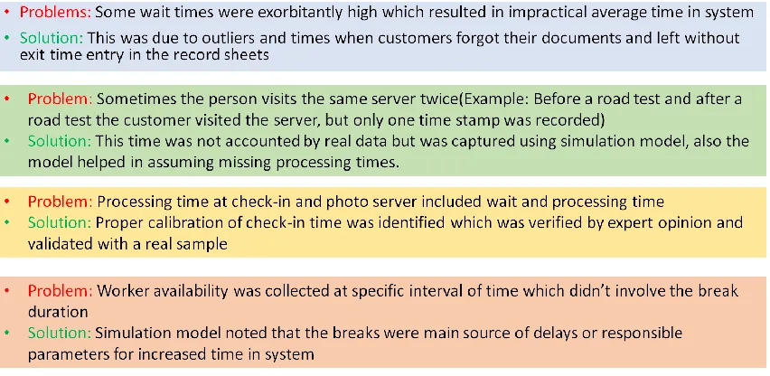
40 3.2.2 Issues with the Data
41 Figure 3.8: Problems with some of the collected data and how simulation served useful in finding solution to the problems
One major difference in collecting data for simulation versus Six Sigma analysis is that Six Sigma often combines processing time and wait time together when the processing time is so small in comparison to wait time. While the simulation team was explicit about needing the actual processing times, some of the data (e.g., greeter processing time) that was collected combined service time (i.e., processing time) and wait time together. However, for the simulation model, the queuing times are calculated and one only needs processing time..
42 passes, he again goes back to the evaluator, which again adds processing time which was not collected. If the data was to be recollected, then there would have been a huge time and money loss to DMV; so, using simulation, certain data was assumed based on some pilot readings and time study to identify the double processing time. This gave a real representation of the system. Therefore, Simulation Modeling can be used as a tool to determine the necessary data and correct any problems in a Measure phase of a DMAIC process.
3.2.3 Input Modeling
Again, the Six Sigma process is not a sequential process, meaning the initial simulation model was built during the beginning of the Analyze phase while the data was being collected as well as identifying any new data that is needed. Once the data is collected, the data needs to be cleaned. After it is cleaned, a data distribution is fitted to the processing times data. In order to fit the data to a distribution, any fitting software as mentioned in Section 2.4.2.2 can be used to fit the distributions. This research utilized the EasyFit™ fitting software because of its flexibility and ability to translate EasyFit™ parameters into the SIMIO™ parameters using the following method:
Collect sample data with sufficient number of data points;
Use the EasyFit™ software to Fit the Distribution;
43
Based on the best distribution by EasyFit™, collect the parameters and create corresponding SIMIO™ expression.
44 Figure 3.9: Fitted Distribution for Other Transaction Customer Type
45 validation via the system was used to model those situations using BetaPert distributions where a minimum, maximum, and most likely case were determined by the team.
Table 3.1: Distributions that Were Used to Model the DMV Variable Description SIMIO™ Random Expression Determined
State IDs LogLogistic(3.33, 4.16) Fitted
License without any test
Lognormal(1.7425, 0.64473 Fitted License before Road
Test
3 Expert Opinion
License After Road Test
Lognormal(1.786426, 0.839898) + .27
Fitted License after Road test
and written Test
Lognormal(1.786426, 0.839898) + .27
Fitted License after written
test before road test
Lognormal(1.786426, 0.839898) + .27
Expert Opinion Before Written Test Lognormal(1.786426, 0.839898) +
.27
Expert Opinion Written test/Computer
Test
Lognormal(1.786426, 0.839898) + .27
Fitted Written CDL JohnsonSB(0.18151, 0.41229,
0.68887, 13.23587)
Fitted
Permits Lognormal(0.62625, 1.8545) Fitted
Appointment Lognormal((1.786426, 0.839898) + .27)
Fitted Others Transactions JohnsonSB(1.0106, 0.63227,
0.68841, 5.9143)
Fitted Before Written
Provisional I
Gamma(3.2009, 1.4328) Fitted
After Written Provisional I
Gamma(3.2009, 1.4328) Fitted
Provisional III Gamma(3.2009, 1.4328) Fitted
Motorcycle Gamma(1.75, 2.8571) Fitted
Reinstate Lognormal(1.786426,0.839898)+.27 Fitted
Road Test Triangular(12.5, 17, 27.5) Fitted
Written Test Poisson(19.8) Fitted
3.3 Analyze Phase
47 3.3.1 Building the Initial Current State Simulation Model of the DMV
The Six Sigma team already knew ahead of time during the Define and Measure phases that Simulation Modeling was going to be used to help identify potential improvements. Therefore, the initial models were built using the detailed process map from Figure 3.1. The Six Sigma team noted three potential problem offices in the state ( Charlotte, Greensboro, and Durham) for potential models. All three offices were visited and observed to aid in the simulation modeling. Also, the Six Sigma team brainstormed potential improvements and wanted the ability to change schedules of personnel, the number of evaluators, etc. Other improvements were discovered after the initial model was built. but these ideas of improvements at this junction helped to shape the model building. Also, the Six Sigma process identifies the metrics used to judge the problem system during the Measure phase which are then used in the simulation model. One advantage of using the DMAIC process in conjunction with simulation rather than Simulation Modeling alone is the identification of the metrics and input variables is built into the methodology.
3.3.2 Simulation tools and software used
49 throughout the simulation and are typically set at the beginning of the simulation for static objects (i.e., Servers, Sinks, Sources, etc.) or set when dynamic objects are created (i.e., Entities, Workers, etc.). State variables on the other hand can have their value changed throughout the run of the simulation.
Because these models are often being built before all the data is collected, it is important to design the model with as much flexibility as possible from the beginning as many things may change. All inputs that could be changed were modeled as properties or input parameters to the simulation model (i.e., number of workers, passing rates of the written and road test, the processing times of the various steps). No input was hard coded with in the properties of the objects or with in the process logic. Using SIMIO™ data tables to model customer types, worker schedules, appointments, etc. was also employed so these could be easily changed and will be described below.
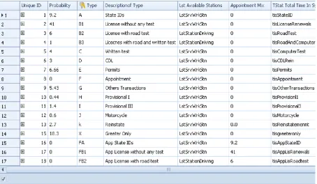
3.3.2.1 Data
Since the offices are basically the same except for layout and number of workstations, the models need to be data driven to reflect the different customer mix, changes in processing times, etc. Table 3.2 shows the fields of the customer type table while Figure 3.10 shows a portion of the actual SIMIO™ table for the customer mix. As can be seen there are basically fourteen basically different classes of DMV customers with a repeat for appointment customers. To facilitate the use of the same processes for both regular customers and appointment customers throughout the model, the same table was needed. As can be seen, the
Probability field is zero for appointment customers so they are not generated by the normal
50 only appointment customers are created by the appointment process. To facilitate the DMV’s desire to route certain classes of customers to certain workstations (for example., only people needing road test are sent to the first three evaluators who are more experienced), the
LstAvailableWorkstations field specifies which list of workstations the particular customer
should use to route to the next available evaluator at a workstation. Table 3.2: Fields of the Customer Table
Column Description
UniqueID Unique identifier and row determination
Probability Customer Mix Percentage used to determine customer type upon arrival (Type As occur 9.2 percent of the time) Type Different Classes of Customer and the primary key. Note
appointment types beging with F DescriptionofType Description of the Customer Class LstAvailableStations The workstation they can be sent to.
AppointmentMix Same Customer mix percentage but for customers with appointment as they have higher priority than nonappointment customers.
TStatTotalTimeInSystem Tally statistics to collect Time in system for all individual types of transaction
51 Figure 3.10: Portion of the SIMIO™ Customer Data Table
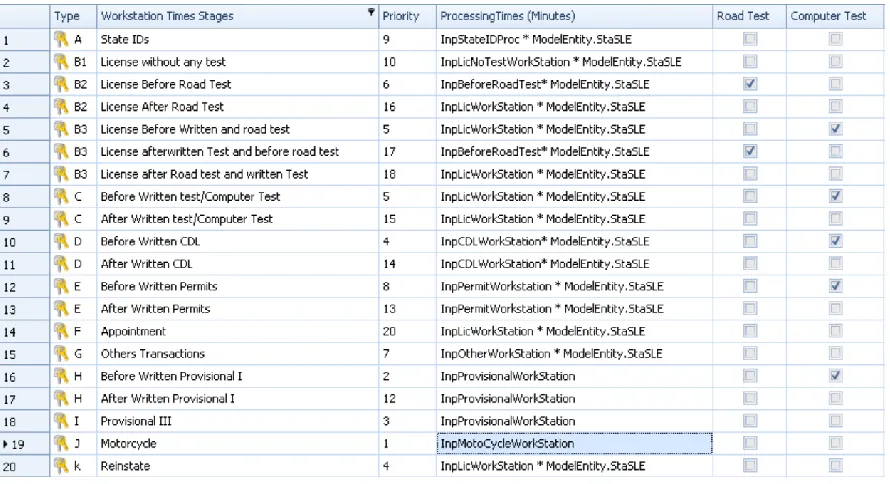
52 checked mean the customer needs to take a road test or a computer test. Figure 3.12: Customer Processing Table as a Related Table to the Customer Table shows the relational table which relates each customer type to another table. Here customer type is assigned as a primary key. Further, the row Lst Available Stations shows the available stations for particular type of transaction. For example, workstation 2 and workstation 3 take customers who want to take a road test while other workstations evaluate customers for any other transaction. This is done by adding the workstations in a different list.
Table 3.3: Customer Processing Time Table
: Description
Type Type of Customer (Foreign Key)
WorkstationTimesStages Description of which stage of the customer Priority Priority associated with the customer at this stage
ProcessingTimes The processing time associated with the customer type for this stage
RoadTest Is this stage a road test?
ComputerTest Is this stage a computer test?
53 Figure 3.11: Customer Processing Time and Priority Table
Figure 3.12: Customer Processing Table as a Related Table to the Customer Table 3.3.2.2 Modeling DMV Evaluators
54 taker or to take customers on road tests. Therefore, the SIMIO™ Worker moveable resource object will be used but modified to create a new worker to help with the DMV scenario. Table 3.4 describes the additional properties and state variables added to the standard Worker object. Currently, the Worker has the ability to specify a home node so that when the worker goes idle or goes off shift, the Worker will move to that home location. However, in the DMV situation these two abilities needed to send them to different locations. If idle the worker would return to the assigned workstation but off shift the worker would leave the system as well as not be available. To handle this situation, two new state variables and a property are needed to switch the home node to the actual home node if the is going on shift but switch it to the off shift location node if the worker is going off shift. These changes are implemented in a modified OnCapacity Changed process event of the Worker processes.
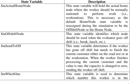
Table 3.4: Added State Variables and Properties of the Worker Object
State Variable Description
StaActualHomeNode This state variable will hold the actual home node where the worker should be normally stationed to perform work (i.e., workstation). This is necessary as the default HomeNode state variable is reassigned during the simulation to be the OffShiftNode or the Home Node.
StaOffshiftNode This state variable identifies which node should be used when the evaluator goes off shift (i.e., break, lunch, etc.).
StaSendToOff This state variable determines if the worker
has gone off shift but needs to finish the current customer either on the road test or at the workstation. When the worker finishes processing the current customer and the value is one, the capacity is changed to zero, sending the worker off shift.
StaWhichOne This state variable is used to determine
55 population of workers.
InitialOffShiftNode The property allows the modeler to specify the off shift node.
LatenessTime This property allows the modeler to specify
the lateness distribution to model the small deviations of workers arriving on time.
AbsentProbability This property determines the absent
probability of whether the worker does not show up for a reason.
The modified Worker object is being used to model the DMV evaluators. In order to allow the decision maker to specify the number of evaluators that are available on a given day, one instance of the worker object will be used and a Source will be used to create that number of evaluators. Since only one worker object is instantiated, only one home node for all the workers is created, which is not the case for the DMV. To be flexible, the table of home nodes seen in Figure 3.13 is used to specify the home node for each of the evaluators where the Which Col field is linked to the StaWhichOne state variable of the worker described in Table 3.4.
56 Figure 3.14 shows the process that is executed each time a Worker is created from the source SrcWorker. The first Assign step assigns which worker number (i.e., first worker receives a value of one) to the StaWhichone state variable of the worker. Again, the state variable allows one to determine this worker out of the population of workers. The next Assign step assigns the standard Home Node state variable the home location from the appropriate row from the home table seen in Figure 3.13. Next the process assigns the actual home node for the worker to be the same, as the home node as the home node state variable will be changed when the worker goes off shift. Finally, the worker is sent to the home node to begin the simulation.
Figure 3.14: Process Executed When each Worker is Created
57 for these properties can be run and determine when is the best time for workers to start. Further, the lunch times were optimized to decrease the average time in system during lunch hours using staggered scheduling pattern for lunch hours. Because the table is time indexed, the process in Figure 3.16 will be invoked at the beginning of each time interval (i.e., each half hour). First, the process determines the current row of the table. Next the Search step is used to loop through all workers in the population and assign the capacity associated with that worker based on the StaWhichOne state variable.
Figure 3.15: Worker Schedule Table
58 Figure 3.17 shows the process logic used for workers to wait in the system until the number of customers in the system is zero after 5:00 PM. If the worker goes off shift at or after 5:00 pm and the number of customers in the system is greater than zero, the system will change the capacity back to one, placing the worker back on shift. Then after ten minutes the process will recheck to see if customers still are present in the system. Once the criteria is false then the system will shut down.
Figure 3.17: Waiting for the Number in System to go to Zero After 5:00 PM 3.3.2.3 Modifying the Server and Model Entity
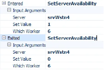
59 seen in Figure 3.19 is used for all workstation nodes and workers. This process is used by assigning worker and server workstation along with the value as seen in Figure 3.18. The process first decides if his is the correct worker. If this is true, then it sets the new server’s StaAvailable state variable to zero or one depending on the value passed to it. If the server is available, then worker is told to allocate itself to the set of customers.
Figure 3.18: Specifying the SetServerAvailability Process on the Entering and Exiting of a Node
Figure 3.19: Set Server Availability Generic Process
60 Table 3.5: Added State Variables of the ModelEntity
State Variable Description
StaPass This state variable is used to assign whether
a customer has passed or failed the written test or eye/sign test where a value of one indicates a pass.
StawhichWrkerSeized This state variable identifies which worker is processing the model entity (customer) at a workstation. The state variable is used to request the same evaluator for the road test who has seen the customer at the workstation.
StaSLE A value of 1.2 indicates that English is a
second language for this customer; otherwise it is set to one. It generally takes 20% longer to deal with customers who are not native English speakers.
StaRoadFail This state variable is used to assign whether
a customer has passed or failed the road test where a value of one indicates a pass.
3.3.2.4 Greeter and Photo Area
62 Figure 3.20: Process to Reject Customer’s Request
3.3.2.5 Modeling the Customer Behavior at Workstation
Figure 3.21 shows the two parameterized processes when customers enter and exit a workstation. The EnteringtheWorkstation process is triggered when the entity enters the workstation. The process is passed which evaluator to seize and where the evaluator should be moved to. The Assign step assigns the ID of the evaluator that is processing the customer to a state variable which will ensure the same evaluator does the road test if required.
After processing the customer at the workstation, the OutputExitedFromWorkstation
63 the step for incrementing the sequence (i.e., linking to the next row in the related customer processing table seen in Figure 3.12) which sets the next processing time as well as changes the priority level. The next step, Execute, moves the worker (i.e., evaluator) with the customer outside to perform the road test without releasing the evaluator. If the next sequence is not a road test (if no road test is needed or the road test has already been performed), the customer destination node is set to the node leading to the either the photo station or the exit if the customer has failed any of the tests. If the evaluator went off shift while transporting the customer for the road test (i.e., the StaSendToOff of the worker is set to one), then the capacity of the worker is set to zero, sending it off shift before the evaluator is released back to allow for service. If the customer failed either the written or road test, then the overall StaPass is set to zero; otherwise, the eye and sign test is done which determines if the customer has passed all requirements.
64 3.3.2.6 Modeling and Animating the Road Test
65 changes the person into a car for animation purposes by searching the ride queue of the transporter to access the customer.
Figure 3.22: Customer Reaches the Outside for the Road Test
Figure 3.23: Changing the Picture to look like a Car
66 Figure 3.24: Customer and Evaluator Arrive Back to Office
3.3.2.7 Balking and System Failure Reneging Logic
In a DMV office, people arrive and get in the main check-in queue. Suppose there are more than a certain number of people present in the queue, and the customers do not wait in queue but instead just leave/balk from the system. This decision of not entering the queue based on the length of the queue is called balking. Figure 3.25 shows the balking logic used for customers entering the DMV. The process will check to see if the number waiting in the check-in line plus those in the waiting area is greater than or equal to a random balk number (e.g., InpCheckInBalk or Pert(20, 25, 30)). If the number in the system exceeds the input balk number, the customer will leave the system; otherwise it enters the check-in queue.
Figure 3.25: Balking Logic Process Diagram