ABSTRACT
SAKHAEI FAR, MARYAM SADAT. Development of New Dynamic Modulus (|E*|) Predictive Models for Hot Mix Asphalt Mixtures. (Under the direction of Dr. Y. Richard Kim).
This Ph.D. dissertation presents the findings of a research program that was conducted to develop a new, robust, and effective set of dynamic modulus (|E*|) predictive models for hot mix asphalt (HMA) mixtures. These models are capable of implementing different types of mixture and binder properties, i.e., resilient modulus (MR), viscosity(η), and binder shear
modulus (|G*|) as its primary input data. Of equal significance was being capable to estimate changes in modulus as a function of changes in mixture volumetric properties, aggregate gradation, binder properties, test conditions including temperature and loading frequency (time) for various lab results based on different test protocols measurements.
The dynamic modulus, |E*|, is a fundamental property that defines the strain response characteristics of asphalt concrete mixtures as a function of loading rate and temperature. The significance of this material property is three-fold. First, it is one of the primary material property inputs in the Mechanistic Empirical Pavement Design Guide (MEPDG) and software developed by NCHRP Project 1-37A. The MEPDG uses a “master curve” and time-temperature shift factors in its internal computations of modulus. In the MEPDG, the master curve is constructed using a hierarchical structure of inputs ranging from estimates based on mixture volumetric properties and binder tests to full scale mixture dynamic modulus testing. Second, the |E*| is one of the primary properties measured in the Asphalt Mixture Performance Test (AMPT) protocol that complements the volumetric mix design. Third, the |E*| is one of the fundamental linear viscoelastic (LVE) material properties that can be used in advanced pavement response models that are based on viscoelasticity
(AMPT) and AASHTO TP-62 under different aging conditions. The data also consist of binder shear moduli values measured under different aging conditions.
In spite of the demonstrated significance of the |E*|, it is not included in the current long-term pavement performance (LTPP) materials tables. Therefore, a joint study including NCSU researchers and Nichols Consulting Engineers was conducted to populate the LTPP layers with |E*| values and some of the findings are presented in this dissertation. As such, the objective of the dynamic modulus project was to use readily available binder, volumetric, and resilient material properties in the LTPP database to develop |E*| estimates. A part of the research presented in this dissertation provides a thorough review of existing prediction models. In addition, several models have been developed using Artificial Neural Networks (ANNs) for use in this project. Included in this study are assessments of each model, quality control checks applied to the data, and the final structure and format of the dynamic modulus data added to the LTPP database. A program was also developed by the researchers involved in this project at NCSU to assist in populating the LTPP database.
The comprehensive study completed at NCSU for populating the LTPP layers with dynamic modulus values resulted in assembling a numerous |E*| and corresponding binder |G*| test measurements. This extensive master database was then utilized to develop a new set of rational, unbiased and accurate |E*| closed-form models. Two of the proposed models are capable of accurately estimating |E*| of HMA mixtures over the entire range of customarily used testing conditions. In addition to that a set of five different regression models were developed and calibrated for typical temperatures recommended in AASHTO TP-62 test protocol including -10°, 4.4°, 21.1°, 37.8°, and 54.4 °C.
Development of New Dynamic Modulus (|E*|) Predictive Models for Hot Mix Asphalt Mixtures
by
Maryam Sadat Sakhaei Far
A dissertation submitted to the Graduate Faculty of North Carolina State University
in partial fulfillment of the requirements for the degree of
Doctor of Philosophy
Civil Engineering
Raleigh, North Carolina 2011
APPROVED BY:
_______________________________ ______________________________ Dr. Y. Richard Kim Dr. S. Ranji Ranjithan
Chair of the Advisory Committee Advisory Committee
________________________________ ______________________________
Dr. Murthy N.Guddati Dr. Roy H. Borden
Advisory Committee member Advisory Committee member
________________________________ Dr. Subhashis Ghoshal
ii DEDICATION
iii BIOGRAPHY
iv
ACKNOWLEDGMENTS
It would like to offer my profound appreciation and gratitude to all organizations and individuals who made my graduate studies a great opportunity for my professional and personal growth.
I would like to thank Federal Highway Administration who provided the opportunity to start the research to populate the Long Term Pavement Performance (LTPP) database with dynamic modulus values in collaboration with Nichols Consulting Engineers (NCE). I would also thank Mr. Newton Jackson and Jason Puccinelli from NCE and Larry Wiser the project manger from FHWA for their help and collaboration. I also would like to thank Federal Highway Administration for the support they provided for this work under Project No. DTFH61-02-D-00139-Task Order #10. It should be mentioned that the views and conclusions contained in this document are those of the author and should not be interpreted as necessarily representing the official policies, either expressed or implied of the FHWA. I also gratefully acknowledge the support from Southern Transportation Center, and the help from Dr. Ramon Bonaquist at AAT, Dr. Michael Harnsberger at WRI, and Dr. Raj Dongre at the FHWA-TFHRC in providing data for the database assembled in this study.
The support of my committee members, Dr. S. Ranji Ranjithan, Dr. Murthy N. Guddati, Dr. Roy H. Borden and Dr. Subhashis Ghoshal cannot be overlooked. Their generous support and guidance was a tremendous asset towards accomplishing this work. I also would like to extend my thanks to Mr. B. Shane Underwood for his time and help at different stages of progress in the LTPP dynamic modulus project, and from whom I learned a lot during my Ph.D program. I also thank Dr. Sankar Arumugam and Dr. Kumar Mahinthakumar for the light they shed in the last stages of this research.
v
I would like to offer my most sincere thanks to Prof. Y. Richard Kim who advised me tirelessly in both academic and personal levels through my research work. His academic excellence has always inspired me to improve my work, and his mentorship has undoubtedly had an immense effect on my personality and career. Thank You.
To my dear husband Dr. Amir Ardalan Mosavi, thank you for your love and endless encouragement. Accomplishing this work would not be possible without your daily help and support.
vi
TABLE OF CONTENTS
Chapter 1: Introduction ………..…….………. 1
1.1. Executive summary………. 1
1.2. Scope and organization of the dissertation………..… 1
Chapter 2: Literature Review………..……...…..…... 8
2.1. Predictive models ……..………..………..………..……..………..… 8
2.1.1. Original Witczak Equation (NCHRP 1-37A) ……...……… 9
2.1.2. Modified Witczak Equation Based on |G*| (NCHRP 1-40D) ..…….………....… 10
2.1.3. Hirsch Model ..……...………..……...………...……….… 12
2.1.4. Law of Mixtures Parallel Model (Al-Khateeb Model) …….……...……….…… 13
2.1.5. ANN Models ….……...…………..….……...……..…….……...…………...… 14
2.1.6. Regression Model ….……...…………..…….……...…………..…...…...……… 15
2.1.7. Summary of Input Variables ….……...…………..…….…….………..…….….. 15
2.2. Binder properties ….……...………..…….……...…………..…….……...………… 17
2.2.1. Shear Modulus ….……...…………..…….……...…………..…….………..….. 17
2.2.2. Viscosity ….……...…………..…….……...…………..…….…...……….. 17
2.2.2.1. Temperature Susceptibility Relationship ….……...…………..………. 18
2.2.2.2. Ring and Ball Temperature ….……...…………..…….……...……..……….. 20
2.2.2.3. Penetration ….……...…………..…….……...…………..…….……...……... 20
2.2.2.4. Absolute Viscosity ….……...…………..…….……...…………..………….. 20
2.2.2.5. Kinematic Viscosity ….……...…………..…….……...………... 21
2.2.2.6. Example Problem ….……...…………..…….……...……….………... 21
2.2.2.7. Typical Values for Purchase Specification Grade ….……...………..… 22
Chapter 3: Database ….……...…………..…….……...………..……...…… 24
3.1. Introduction ….……...…………..…….……...…………..…….…...……....………. 24
vii
3.3. Binder Databases ….……...…………..…….……...………...…...……….…… 32
3.4. Mixture Databases ….……...…………..…….……...…………..…….….…...…… 38
Chapter 4: Evaluation of the |E*| Predictive Models ….……...………...…….… 56
4.1. Ann structure used in this study ….……...………..…….……...………..….… 56
4.2. Evaluation of Binder |G*|-Based models ….……...…………..…….…….….…...… 58
4.3. Viscosity-Based ANN.……...…………..…….……...………...…....… 75
Chapter 5: AMPT versus TP-62 ….……...………..…….………....……...… 83
5.1. Verification of AMPT and TP-62 differences ….……...………...………...… 83
5.2. Comparison of AMPT and TP-62 Protocols with the Available Database ….…….... 85
5.3. Evaluation of AMPT versus TP-62 Protocols using ANN Model ….……...…….… 100
Chapter 6: Artificial Neural Network |E*| Models for Populating the LTPP Database110 6.1 MR ANN Model ….……...…………..…….……...…………..……...…...… 113
6.1.1. Forward Modeling ….……...…………..……....………...… 114
6.1.2. ANN Model |E*| Backcalculation ….……...……….……...………….…...… 126
6.2. VV ANN Model ….……...…………..…….……...…….………...……....…... 128
6.3. GV ANN Model ….……...…………..…….……...……..……….…....…...… 131
6.4. Other ANN Models ….……...…………..…….……...…….………..………...… 133
6.5. Error Assessment ….……...…………..…….……...………….………...…...…. 134
6.6. ANN model factors ….……...…………...……...…………..………....… 136
6.6.1. MR-Based ANN (MR ANN) ….……...……..…….……...………...……... 140
6.6.2. Viscosity-Based ANN (VV ANN) ….……...……..…….……...…..……..…… 146
6.6.3. |G*|-Based ANN (GV ANN) ….……...……..…….……...…………....…...… 151
Chapter 7: Prediction of |E*| for LTPP Layers ….……...………...….…..…...… 155
7.1. Model Prioritization and Decision Tree Development ….……...………...…...… 155
7.2. Data Quality Control ….……...…………..…….……...………….…....…....…..… 156
viii
8.1. Introduction ….……...…………..…….……...………..…...…..…....…..… 180
8.2. Objective ….……...…………..…….….……...………...………. 183
8.3. Database …….….……...…………..…….…….….…...…………..………….……. 183
8.3.1. Calibration Database …….….……..……..…….…….….……...……...……. 184
8.3.2. Verification Database …….…....…………..…….…….….……..……..…….... 186
8.4. Regression models …….….……...…………..…….…….….…….………..… 187
8.4.1. Statistical Modeling Techniques …….….……...……….….…….….………… 187
8.4.1.1. Correlation Analysis …….….……...…………..……...…….….….………….. 189
8.4.1.2. Stepwise Regression Analysis …….….……...…………..……...………. 189
8.4.1.3. Principal Component …….….……...…………..……...…….….….…………. 190
8.4.2. First Modeling Approach …….….……...……..…….…….….…....…….….… 191
8.4.2.1. Mixture Mastercurve Construction …….….……...…………..……...……. 193
8.4.2.2. Binder Mastercurve Construction …….….……...………….……… 194
8.4.2.3. Model Formulation …….….……...…………..…….…….….………..…… 196
8.4.2.4. Splitting Function Method.……...…………..…….…….….………..…… 199
8.4.3. Second Modeling Approach …….….…………..……….……...…… 206
8.4.4. Sub-Models …….….……...…………..…………..………..…..…..….………. 208
8.4.5. Predictor Variables Used in the New Dynamic Modulus Model Development... 209
8.4.6. Multivariate Correlation Analysis …….….……..……..………....………. 210
8.4.7. Optimization of the α and β Sub-Models …….….…………..………..…. 213
8.4.8. Model Selection …….….……...……….….……...………..……..… 219
8.5. Model performance …….….……...…………..…….…….….……...………..…… 234
8.6. Individual Temperature-Based Models …….….……...………..………. 239
8.6.1. Statement of Need …….….……...…….…….….……...………....………….... 239
8.6.2. Development of Individual Temperature-Based Models ……….…... 241
8.6.3. Model Performance …….….……...………..………..……...………. 254
Chapter 9: Conclusions and Recommendations ….……...……..…...……… 266
9.1. Conclusions …….….……...………..………. ……….……….……… 266
ix
x
LIST OF FIGURES
Figure 1.1. Modulus prediction model decision tree………..… 6 Figure 2.1. A-VTS relationship. ………..… 19 Figure 3.1. Comparison between the Witczak predictive model and measured |G*| values,
using 8,940 data points from the Witczak binder database used to develop the |G*| model in arithmetic scale………. 28 Figure 3.2. Comparison between the Witczak predictive model and measured |G*| values,
using 8,940 data points from the Witczak binder database used to develop the |G*| model in logarithmic scale………...……... 28 Figure 3.3. Comparison between the Witczak predictive model and measured δb, using 8,940
data points from the Witczak binder database used to develop the δb model. …….29 Figure 3.4. Comparison between the Witczak predictive model and measured |G*| values,
using Citgo binders in the NCDOT database in arithmetic scale. ………29 Figure 3.5. Comparison between the Witczak predictive model and measured |G*| values,
using Citgo binders in the NCDOT database in logarithmic scale. ……… 30 Figure 4.1. Prediction of the processed Witczak, FHWA (I), FHWA (II), NCDOT (I),
NCDOT (II), WRI and Citgo databases using modified Witczak in arithmetic scale. ………62 Figure 4.2. Prediction of the processed Witczak, FHWA (I), FHWA (II), NCDOT (I),
NCDOT (II), WRI and Citgo databases using modified Witczak in logarithmic scale………. 62 Figure 4.3. Prediction of the processed Witczak, FHWA (I), FHWA (II), NCDOT (I),
NCDOT (II), WRI and Citgo databases using Hirsch model in arithmetic
scale………. 63 Figure 4.4. Prediction of the processed Witczak, FHWA (I), FHWA (II), NCDOT (I),
NCDOT (II), WRI and Citgo databases using Hirsch model in logarithmic scale. 63 Figure 4.5. Prediction of the processed Witczak, FHWA (I), FHWA (II), NCDOT (I),
NCDOT (II), WRI and Citgo databases using Al-Khateeb model in arithmetic scale. ………...… 64 Figure 4.6. Prediction of the processed Witczak, FHWA (I), FHWA (II), NCDOT (I),
NCDOT (II), WRI and Citgo databases using Al-Khateeb model in logarithmic scale. ………..……. 64 Figure 4.7. Prediction of training data containing processed Witczak, FHWA (I), NCDOT (I)
xi
Figure 4.8. Prediction of training data containing processed Witczak, FHWA (I), NCDOT (I) and WRI databases using G-GR pANN in logarithmic scale. ………67 Figure 4.9. Prediction of training data containing processed Witczak, FHWA (I), NCDOT (I)
and WRI databases using G-V pANN in arithmetic scale………. 68 Figure 4.10. Prediction of training data containing processed Witczak, FHWA (I), NCDOT (I)
and WRI databases using G-V pANN in logarithmic scale. …………..………… 68 Figure 4.11. Predicted moduli using G-GR pANN and modified Witczak models for FHWA
(II) database in arithmetic scale. ………...… 69 Figure 4.12. Predicted moduli using G-GR pANN and modified Witczak models for FHWA
(II) database in logarithmic scale. ………..…… 69 Figure 4.13. Predicted moduli using G-V pANN and Hirsch models for FHWA (II) database
in arithmetic scale. ………..… 70 Figure 4.14. Predicted moduli using G-V pANN and Hirsch models for FHWA (II) database
in logarithmic scale. ………..… 70 Figure 4.15. Predicted moduli using G-GR pANN and modified Witczak models for NCDOT
(II) database in arithmetic scale………..…. 71 Figure 4.16. Predicted moduli using G-GR pANN and modified Witczak models for NCDOT
(II) database in logarithmic scale……….71 Figure 4.17. Predicted moduli using G-V pANN and Hirsch models for NCDOT (II) database
in arithmetic scale……….72 Figure 4.18. Predicted moduli using G-V pANN and Hirsch models for NCDOT (II) database
in logarithmic scale. ……….………. 72 Figure 4.19. Predicted moduli using G-GR pANN and modified Witczak models for Citgo
database in arithmetic scale. ………..…. 73 Figure 4.20. Predicted moduli using G-GR pANN and modified Witczak models for Citgo
database in logarithmic scale……….……….…… 73 Figure 4.21. Predicted moduli using G-V pANN and Hirsch models for Citgo database in
arithmetic scale. ………..…… 74 Figure 4.22. Predicted moduli using G-V pANN and Hirsch models for Citgo database in
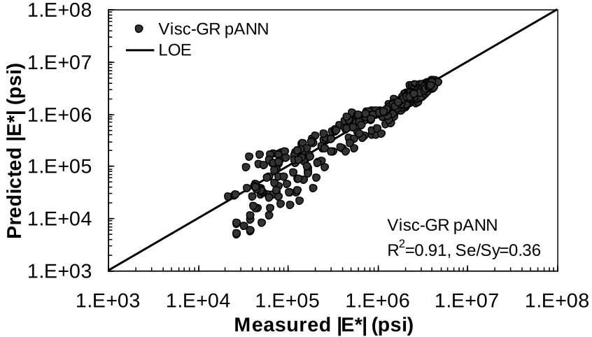
logarithmic scale………..….74 Figure 4.23. Prediction of training data containing Witczak, FHWA (I) and NCDOT (I)
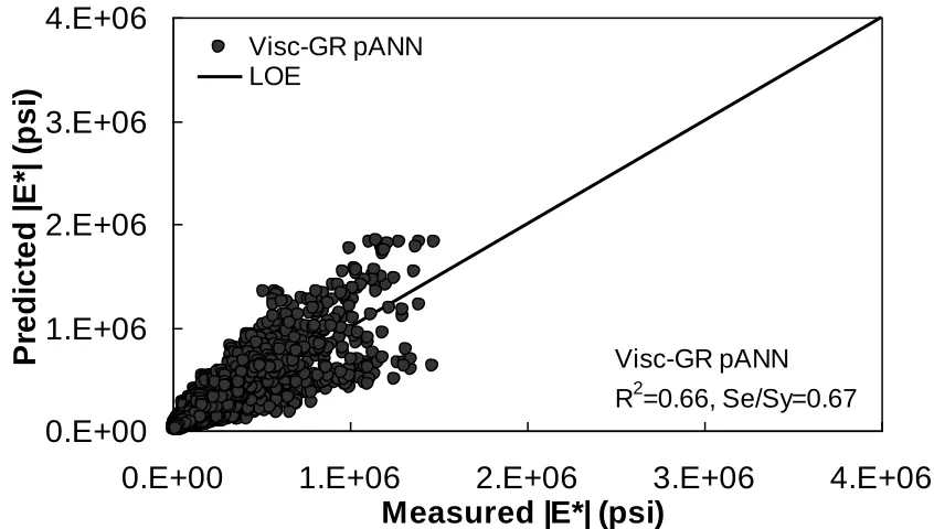
databases using Visc-GR pANN in arithmetic scale. ……….………….... 77 Figure 4.24. Prediction of training data containing Witczak, FHWA (I) and NCDOT (I)
xii
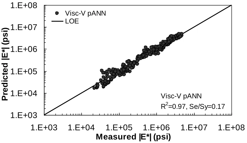
Figure 4.25. Prediction of training data containing Witczak, FHWA (I) and NCDOT (I)
databases using Visc-V pANN in arithmetic scale. ………78 Figure 4.26. Prediction of training data containing Witczak, FHWA (I) and NCDOT (I)
databases using Visc-V pANN in logarithmic scale……….…. 78 Figure 4.27. Predicted moduli using Visc-GR pANN model for FHWA (II) database in
arithmetic scale………....…... 79 Figure 4.28. Predicted moduli using Visc-GR pANN model for FHWA (II) database in
logarithmic scale………. 79 Figure 4.29. Predicted moduli using Visc-V pANN model for FHWA (II) database in
arithmetic scale………..…. 80 Figure 4.30. Predicted moduli using Visc-V pANN model for FHWA (II) database in
logarithmic scale. ……….…….…. 80 Figure 4.31. Predicted moduli using Visc-GR pANN model for NCDOT (II) database in
arithmetic scale. ………. 81 Figure 4.32. Predicted moduli using Visc-GR pANN model for NCDOT (II) database in
logarithmic scale. ……….…. 81 Figure 4.33. Predicted moduli using Visc-V pANN model for NCDOT (II) database in
arithmetic scale.……… ………. 82 Figure 4.34. Predicted moduli using Visc-V pANN model for NCDOT (II) database in
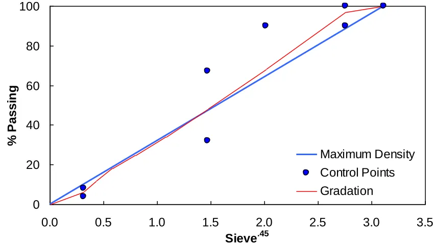
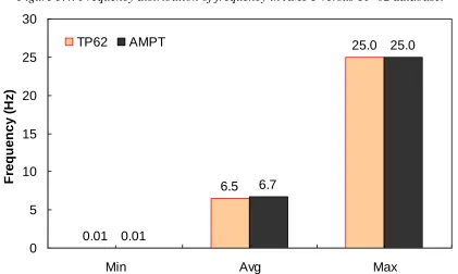
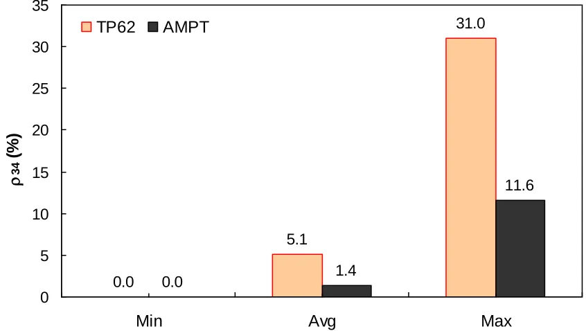
logarithmic scale. ………..…. 82 Figure 5.1. Test mixture gradation………..……. 84 Figure 5.2. Frequency distribution of temperature in AMPT versus TP-62 database. ……… 86 Figure 5.3. Range of temperature in AMPT versus TP-62 database. ……….… 86 Figure 5.4. Frequency distribution of frequency in AMPT versus TP-62 database. ……..… 87 Figure 5.5. Range of loading frequency in AMPT versus TP-62 database. ……… 87 Figure 5.6. Frequency distribution of percent retained on 3/4" sieve (p34) in AMPT versus
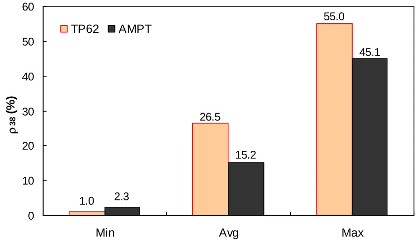
TP-62 database. ……….88 Figure 5.7. Range of percent retained on 3/4" sieve (p34) in AMPT versus TP-62. ………… 88 Figure 5.8. Frequency distribution of percent retained on 3/8" sieve (p38) in AMPT versus
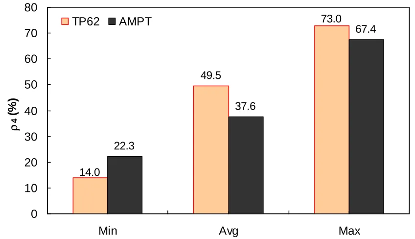
TP-62 database. ………..………. 89 Figure 5.9. Range of percent retained on 3/8" sieve (p38) in AMPT versus TP-62 database... 89 Figure 5.10. Frequency distribution of percent retained on #4 sieve (p4) in AMPT versus
xiii
Figure 5.12. Frequency distribution of percent passing #200 sieve (p200) in AMPT versus TP-62 database. ……….………91 Figure 5.13. Range of percent passing #200 sieve (p200) in AMPT versus TP-62 database. …91 Figure 14. Frequency distribution of specimen air voids in AMPT versus TP-62 database.... 92 Figure 5.15. Range of specimen air voids in AMPT versus TP-62 database. ………..……… 92 Figure 5.16. Frequency distribution of effective binder volume in AMPT versus TP-62
database. ……….……… 93 Figure 5.17. Range of effective binder volume in AMPT versus TP-62 database. …….…… 93 Figure 5.18. Frequency distribution of voids in mineral aggregates in AMPT versus TP-62
database. ……….………….…94 Figure 5.19. Range of voids in mineral aggregates in AMPT versus TP-62 database. ……… 94 Figure 5.20. Frequency distribution of voids filled with asphalt in AMPT versus TP-62
database. ……….……….…...… 95 Figure 5.21. Range of voids filled with asphalt in AMPT versus TP-62 database. ………… 95 Figure 5.22. Frequency distribution of |G*| in AMPT versus TP-62 database. ………96 Figure 5.23. Range of |G*| in AMPT versus TP-62 database. ……… 96 Figure 5.24. Percentage of difference between AMPT versus TP-62 database based on similar
ranges of different variables at 4.4°C. ………... 97 Figure 5.25. Percentage of difference between AMPT versus TP-62 database based on similar
ranges of different variables at 21.1°C. ………..…… 98 Figure 5.26. Percentage of difference between AMPT versus TP-62 database based on similar
ranges of different variables at 37.8°C. ………..……… 98 Figure 5.27. Percentage of difference between AMPT versus TP-62 database based on similar
ranges of different variables at 54.0°C. ………99 Figure 5.28. Percentage of difference between AMPT versus TP-62 database based on similar
ranges of different variables at 54.4°C. ………..………… 99 Figure 5.29. Prediction of the combination of AMPT and TP-62 data using (a) modified
Witczak and G-GR pANN (b) Hirsch (c) Al-Khateeb models in arithmetic and
logarithmic scales. ………104 Figure 5.30. Prediction of the AMPT data using (a) modified Witczak and AMPT pANN (b)
Hirsch (c) Al-Khateeb models in arithmetic and logarithmic scales. ………105 Figure 5.31. Prediction of the TP-62 data using (a) modified Witczak and TP-62 pANN (b)
xiv
Figure 5.32. Prediction of the FHWA (II) data using (a) modified Witczak and G-GR pANN (b)AMP pANN and TP-62 pANN, (c) Hirsch, and (d) Al-Khateeb models in arithmetic and logarithmic scales………. 107 Figure 5.33. Prediction of the NCDOT (II) data using (a) modified Witczak and G-GR pANN
(b)AMP pANN and TP-62 pANN, (c) Hirsch, and (d) Al-Khateeb models in arithmetic and logarithmic scales………..…… 108 Figure 5.34. Prediction of the CITGO data using (a) modified Witczak and G-GR pANN
(b)AMP pANN and TP-62 pANN, (c)Hirsch, and (d) Al-Khateeb models in
arithmetic and logarithmic scales.……… ……….….. 109 Figure 6.1. Network structure used for training the ANN models……….… 113 Figure 6.2. Stress distribution in the IDT specimen subjected to a strip load. ………..…… 116 Figure 6.3. Poisson’s ratio versus reduced time for S12.5C. ……… 121 Figure 6.4. Comparison of predicted and measured MR values for S12.5C mixture. ………124 Figure 6.5. Comparison of predicted and measured MR values for S12.5CM mixture. …… 124 Figure 6.6. Comparison of predicted and measured MR values for S12.5FE mixture. ….… 125 Figure 6.7. Comparison of predicted and measured MR values for B25.0C mixture. …..…. 125 Figure 6.8. MR ANN model using 90% of randomly selected data as training set in arithmetic
scale. ………....… 126 Figure 6.9. MR ANN model using 90% of randomly selected data as training set in
logarithmic scale………..….… 127 Figure 6.10. MR ANN model using 10% of randomly selected data as verification set in
arithmetic scale………. 127 Figure 6.11. MR ANN model using 10% of randomly selected data as verification set in
logarithmic scale………..……. 128 Figure 6.12. VV ANN model using 90% of randomly selected data as training set in
arithmetic scale……….….… 129 Figure 6.13. VV ANN model using 90% of randomly selected data as training set in
logarithmic scale………..……. 129 Figure 6.14. VV ANN model using 10% of randomly selected data as verification set in
arithmetic scale………. 130 Figure 6.15. VV ANN model using 10% of randomly selected data as verification set in
logarithmic scale……….……. 130 Figure 6.16. GV ANN model using 90% of randomly selected data as training set in
xv
Figure 6.17. GV ANN model using 90% of randomly selected data as training set in
logarithmic scale………..………. 132 Figure 6.18. GV ANN model using 10% of randomly selected data as verification set in
arithmetic scale. ……… 132 Figure 6.19. GV ANN model using 10% of randomly selected data as verification set in
logarithmic scale………... 133 Figure 7.1. Decision tree applied to population of LTPP database based on ranking……... 157 Figure 7.2. Example of the effect of a violation of QC #1 for case of MR ANN model in
semi-log scale………. 159 Figure 7.3. Example of the effect of a violation of QC #1 for case of MR ANN model in
log-log scale………..………..….………… 159 Figure 7.4. Example of the effect of a violation of QC #1 for case of VV ANN model in
semi-log scale……….…………...………… 160 Figure 7.5. Example of the effect of a violation of QC #1 for case of VV ANN model in
log-log scale………..…………...………… 160 Figure 7.6. Example of the effect of a violation of QC #1 for case of VV ANN model,
unshifted data. ………..……… 161 Figure 7.7. Example of the effect of a violation of QC #2 in semi-log scale. ………162 Figure 7.8. Example of the effect of a violation of QC #2 in log-log scale. ………….…… 162 Figure 7.9. Example of the effect of a violation of QC #2, unshifted data. ……….. 163 Figure 7.10. Example of the effect of a violation of QC #3 in semi-log scale. ……… 164 Figure 7.11. Example of the effect of a violation of QC #3 in log-log scale. ……… 165 Figure 7.12. Example of the effect of a violation of QC #2, unshifted data. ………….…… 165 Figure 7.13. Example of the effect of a violation of QC #4 in semi-log scale………... 166 Figure 7.14. Example of the effect of a violation of QC #4 in log-log scale. ……… 167 Figure 7.15. Example of the effect of a violation of QC #4, unshifted data. ………….…… 167 Figure 7.16. Example of the effect of a violation of QC #5 in semi-log scale. ……….…… 169 Figure 7.17. Example of the effect of a violation of QC #5 in log-log scale. ……… 169 Figure 7.18. Example of the effect of a violation of QC #4, unshifted data. ………….…… 170 Figure 7.19. The ANN models and their appropriate input and output tables. …………..… 179 Figure 8.1. Predicted modulus values using the CAM-|E*| model without the correction factor
xvi
Figure 8.2. Predicted modulus values using the CAM-|E*| model with correction factor for the NCSU calibration database in: (a) arithmetic and (b) logarithmic scales. ………199 Figure 8.3. Comparison of individual and average t-T shift factor functions for the mixtures
and binders using the NCSU calibration database..……….……..……201 Figure 8.4. Predicted modulus values using the CAM-|E*| model using average shift factors
for the NCSU calibration database in: (a) arithmetic and (b) logarithmic scales...202 Figure 8.5. Comparison of individual and average |G*| mastercurves at 20°C reference
temperature for: (a) the NCSU calibration database and verification databases, (b) 10% of the NCSU database, (c) processed Witczak database, and (d) AMPT
database.……… 205 Figure 8.6. Predicted modulus values using the CAM-|E*| model with average binder
mastercurve and CAM fit using the NCSU calibration database in: (a) arithmetic and (b) logarithmic scales. ……… 206 Figure 8.7. Predicted modulus values using the |E*| sigmoidal model combined with the
binder shear modulus as the time-temperature independent variable using the NCSU calibration database in: (a) arithmetic and (b) logarithmic scales.……… 207 Figure 8.8. Correlation coefficients versus independent variables for (a) α and (b) β
sub-models of closed-form model #1 using the NCSU calibration database..…….… 212 Figure 8.9. Correlation coefficients versus independent variables for (a) α and (b) β
sub-models of closed-form model # 2 using the NCSU calibration database. ……… 213 Figure 8.10. Relationship of terms “α” and “β” of closed-form model #1 with gradation (p34,
p38, p4, p200) and volumetric parameters (Va, Vbeff, VMA, VFA). ……….. 215 Figure 8.11. Relationship of terms “α” and “β”of closed-form model #2 with gradation (p34,
p38, p4, p200) and volumetric parameters (Va, Vbeff, VMA, VFA). …………...… 216 Figure 8.12. (a) Root mean square error (RMSE) and (b) correlation coefficient (R2) from
stepwise regression analysis for the variable terms in sub-model of global model using the NCSU calibration database.……….………… ….……….. 220 Figure 8.13. (a) Root mean square error (RMSE) and (b) correlation coefficient (R2) from
stepwise regression analysis for the variable terms in sub-model of global model using the NCSU calibration database.……….………… ….……….. 221 Figure 8.14. (a) Root mean square error (RMSE) and (b) correlation coefficient (R2) from
stepwise regression analysis for the variable terms in sub-model of the simplified global model using the NCSU calibration database.…… ….……….. 221 Figure 8.15. (a) Root mean square error (RMSE) and (b) correlation coefficient (R2) from
xvii
Figure 8.16. Global model using the NCSU calibration database in arithmetic scale……… 230 Figure 8.17. Global model using the NCSU calibration database in logarithmic scale……. 230 Figure 8.18. The simplified global model using the NCSU calibration database in arithmetic scale……….…….233 Figure 8.19. The simplified global model using the NCSU calibration database in logarithmic scale………..233 Figure 8.20. Predicted modulus values using the modified Witczak model for 90% of the
NCSU database as the verification set in: (a) arithmetic and (b) logarithmic scale. ………...………..235 Figure 8.21. Predicted modulus values using (a) global, (b) simplified global and (c) and the
modified Witczak model for 10% of the NCSU database as the verification set in arithmetic and logarithmic scales. ……… 236 Figure 8.22. Predicted modulus values using (a) global, (b) the simplified global and (c) the
modified Witczak model for the processed Witczak database as the verification set in arithmetic and logarithmic scales. ……… 237 Figure 8.23. Predicted modulus values using (a) global, (b) the simplified global and (c) the
modified Witczak model for the AMPT database as the verification set in: (a) arithmetic and (b) logarithmic scales. ………..……… 238 Figure 8.24. Predicted modulus values using (a) global, (b) the simplified global and (c) the
modified Witczak model for 90% of the NCSU database segregated by
temperature in arithmetic and logarithmic scales. ………....……… 241 Figure 8.25. Relationship of log|E*| versus log|G*| for pilot models #1 and #2 at different
individual temperatures. ………..…….………… 243 Figure 8.26. Correlation coefficients versus independent variables for (a) α and (b) β terms
used in the exponential form of the individual temperature-based pilot model 2 using the NCSU calibration database. ………..……… 245 Figure 8.27. Individual temperature-based pilot model #2 using the NCSU calibration
database in (a) arithmetic and (b) logarithmic scales. ……….. 247 Figure 8.28. Individual temperature-based models using the NCSU calibration database in
arithmetic scale. ……… 252 Figure 8.29. Individual temperature-based models using the NCSU calibration database in
logarithmic scale. ……….………. 253 Figure 8.30. Predicted modulus values using individual temperature-based models, including
xviii
the modified Witczak models for 10% of the NCSU database segregated by
temperature in arithmetic and logarithmic scales. ……… 257 Figure 8.31. Predicted modulus values using individual temperature-based models, including
(a) final model, (b) pilot model 2, and (c) global, (d) the simplified global, and (e) the modified Witczak models for the processed Witczak database segregated by temperature in arithmetic and logarithmic scales. ……… 258 Figure 8.32. Predicted modulus values using individual temperature-based models, including
xix
LIST OF TABLES
Table 2.1. Predictive Relationships for |E*|.………..………… 9
Table 2.2. Model variables. ……….……… 16
Table 2.3. Relationship between asphalt binder grade and viscosity parameters. ……...…… 23
Table 3.1. An Example of Summarized Mixture and Binder Properties in the Original Witczak Database ……… 26
Table 3.2. Summary of |G*| Data Available in the Witczak Binder Database. ……… 33
Table 3.3. Summary of |G*| Data Available in the FHWA Mobile Trailer Database. ……… 34
Table 3.4. Summary of |G*| Data Available in the FHWA TPF-5(019) Binder Database. … 35 Table 3.5. Summary of |G*| Data Available in the NCDOT Binder Database. …………..… 36
Table 3.6. Summary of |G*| Data Available in the Citgo Binder Database. ……… 36
Table 3.7. Summary of |G*| Data Available in the WRI Database. ……… 37
Table 3.8. Summary of |G*| Data Available in the expanded NCSU Binder Database. ….… 38 Table 3.9. Summary of |E*| Data Available in the Processed Witczak Mixture Database. … 40 Table 3.10. Summary of |E*| Data Available in the FHWA(I) Mobile Trailer Mixture Database. ……… 41
Table 3.11. Summary of |E*| Data Available in the FHWA (II) Mobile Trailer Mixture Database. ……… 42
Table 3.12. Summary of |E*| Data Available in the FHWA TPF-5(019) Mixture Database... 43
Table 3.13. Summary of |E*| Data Available in the NCDOT Mixture Database. ……… 44
Table 3.14. Summary of |E*| Data Available in the WRI Database. ………..…… 45
Table 3.15. Summary of |E*| Data Available in the Citgo Mixture Database. ……… 46
Table 3.16. Summary of |E*| Data Available in the expanded NCSU Mixture Database. … 48 Table 3.17. Summary of |E*| Data Available in the Resilient Modulus Database. ………… 49
Table 3.18. Summary of extracted LTPP data. ……… 52
Table 4.1. Description of |G*|-Based ANN Models. ……… .. 66
Table 4.2. Description of Viscosity-Based ANN Models. ……….……. 76
Table 5.1. Test Protocol Summary. ………. 83
xx
xxi
Table 6.26. Wkj2 Matrix Elements for GV ANN (part 1). ……… 152 Table 6.27. Wkj2 Matrix Elements for GV ANN (part 2). ……… 153 Table 6.28. Wkj2 Matrix Elements for GV ANN (part 3). ……… 153 Table 6.29. Bj2 Vector Elements for GV ANN (transposed for convenience). …….……... 154 Table 6.30. Wj3 Vector Elements for GV ANN. ……….……..… 154 Table 6.31. Normalization Parameters for GV ANN. ……… 154 Table 7.1. Input Ranges of different ANN Models. ………..…… 158 Table 7.2. Limiting |E*| Values used for QC #6. ………..…… 171 Table 7.3. Statistics of LTPP Data Populated with |E*|.……….…… 174 Table 7.4. Structure and format of the TST_ESTAR_MASTER Table. ………..…… 176 Table 7.5. Structure and format of the TST_ESTAR_MODULUS Table. …………....…… 176 Table 7.6. Structure and format of the TST_ESTAR_MODULUS_COEFF Table. …….… 177 Table 7.7. Structure and format of the TST_ESTAR_GSTAR_INPUT Table. ……… 177 Table 7.8. Structure and format of the TST_ESTAR_GSTAR_CAM_COEFF Table. ….… 177 Table 7.9. Structure and format of the TST_ESTAR_VOLUM_INPUT Table. ………...… 177 Table 7.10. Structure and format of the TST_ESTAR_VISC_INPUT Table. …………..… 178 Table 7.11. Structure and format of the TST_ESTAR_VISC_MODEL_COEFF Table…… 178 Table 7.12. Structure and format of the TST_ESTAR_MR_INPUT Table. ……….… 178 Table 8.1. Summary of |E*| data available in NCSU calibration mixture database. ….…… 185 Table 8.2. Summary of |E*| data available in NCSU verification mixture database. …….…187 Table 8.3. Correlation matrix for “α”, “β” and independent variable terms of global model
using the NCSU calibration database. ………..… 211 Table 8.4. Correlation matrix for “α”, “β” and independent variable terms of the simplified
model using the NCSU calibration database. ……….……….…….…… 212 Table 8.5. Correlation matrix for “α”, “β” and variable terms of global model using the NCSU
calibration database. ……….…… 218 Table 8.6. Correlation matrix for “α”, “β” and variable terms of the simplified global model
using the NCSU calibration database. ……….…… 218 Table 8.7. Stepwise regression for selecting the closed-form models. ………...……220 Table 8.8. Regression model coefficients and fitness measurements for pilot closed-form
xxii
Table 8.9. Description of the developed closed-form models and their validation statistics.. 235 Table 8.10. Stepwise regression for selecting the individual temperature-based closed-form
models. ……….……… 246 Table 8.11. Relative importance factor for different variables used in “” and “” sub-models
of individual temperature-based model..………...……… 253 Table 8.12. Developed closed-form models and their validation statistics segregated for
Chapter 1: Introduction
1
Chapter 1:
Introduction
1.1.
EXECUTIVE SUMMARY
The dynamic modulus, |E*|, is a fundamental property that defines the stiffness characteristics of hot mix asphalt (HMA) mixtures as a function of loading rate and temperature.
Given the significance of the |E*| in pavement engineering, a part of this research was undertaken to populate the LTPP database with |E*| estimates using material properties currently available for LTPP test sections. In this study, a team consists of the North Carolina State University researchers and Nichols Consulting Engineers evaluated existing models used to estimate |E*| values and additional models that have been developed based on the use of Artificial Neural Networks (ANNs). Using the results of the model evaluation, the team has developed a model selection hierarchy and populated the LTPP database with |E*| estimates at five temperatures and six frequencies as well as shift factors and sigmoidal functions that can be used to construct mastercurves (Kim et al., 2009).
The other part of the research study presented in this dissertation is the outcomes of a study effort for developing a new set of regression models for estimating the |E*| values of HMA mixtures.
1.2.
SCOPE AND ORGANIZATION OF THE DISSERTATION
This dissertation is organized in nine chapters. The proposed new developed models for predicting the dynamic modulus of hot mix asphalt mixtures are discussed in these nine chapters.
time-Chapter 1: Introduction
2
temperature dependency concept that is used for characterizing the behavior of HMA mixture.
The models identified at the outset of this project as potentially suitable for the task at hand were:
1. Original Witczak Equation (NCHRP 1-37A) 2. Modified Witczack |G*| Equation (NCHRP 1-40D) 3. Hirsch Model
4. Law of Mixtures Parallel Model
5. Resilient Modulus (MR)-Based ANN Model
6. Viscosity-Based ANN Model 7. |G*|-Based ANN Model
The existing predictive models (numbers 1 through 4 above) are collectively referred to in this study as the closed-form models. Specific comparisons are drawn regarding their forms and required input parameters.
Chapter 1: Introduction
3
the Witczak database was combined with mixtures from other national projects and efforts undertaken at North Carolina State University (NCSU). This expanded mixture database now includes 22,505 data points.
In addition to compiling a mixture database, binder properties likewise have been compiled into a similarly expansive database. Substantial efforts have been expended for developing the appropriate binder data processing techniques. The required processing varied depending on the type of data available, i.e., |G*|, viscosity or binder grade. The first seven chapters of this dissertation also include the outcomes from a research study to populate the Long Term Pavement Performance (LTPP) database with dynamic modulus values. To achieve this goal the needed information was extracted from LTPP tables and are briefly described in this chapter.
Chapter 4 presents the identification and evaluation of four different existing predictive models that could be used to estimate the |E*| of the LTPP HMA layers. The conclusion from that study is that, although each model has its specific advantages and disadvantages, each was found lacking in its ability to predict |E*| values over the range of temperatures necessary for MEPDG input. Closed-form models are compared using data sets that were not used in the calibration of the respective models. It is found that the law of mixtures parallel model shows a significant bias, but the Hirsch model shows reasonable predictions except for insensitivity under extreme conditions. For the verification database, the Hirsch model shows slightly better statistical predictions than either of the Witczak models. This finding, along with other statistical analyses, eventually led the research team to adopt the Hirsch model input parameters into the viscosity- and |G*|-based ANN models.
Chapter 1: Introduction
4
techniques is that the functional form of the relationship is not needed a priori. Considering that many variables affect the |E*| values and their interaction, the ANN technique may capture complicated nonlinear relationships between the |E*| and other mixture variables better than regression analysis.
Chapter 5 presents the results of assessment of differences in the measured moduli determined from the AMPT and TP-62 protocols. Early in the project, concerns arose because the database combined moduli that had been measured using two different methods, the AASHTO TP-62 protocol and the Asphalt Mixture Performance Tester (AMPT) protocol. A study of the available databases revealed that the mixtures tested according to the AASHTO TP-62 protocol tend to yield higher moduli values than similar mixtures tested using the AMPT protocol. Statistical analysis to assess the significance of the difference was not performed, but the two data ranges do tend to overlap, which suggests a lack of statistical significance in their differences. A limited experimental study wherein the modulus of a single mixture was measured using the two protocols was also conducted. The study shows a statistically significant difference of about 12 percent in the measured moduli across all studied temperatures and frequencies (Kim et al., 2009). However, in light of the fact that both protocols are readily available, and that without a more comprehensive and controlled experimental program neither of the available protocols can be discounted, the decision was made to include all available data, both AMPT and TP-62, in the calibration process.
In addition, appropriate portions of each TP-62 and AMPT databases having the same aging conditions are considered to develop predictive models. The results of this study showed that the |E*| values measured by the AMPT protocol seem to be slightly different from those measured by the TP-62 protocol. As such, the |E*| predictive models developed using TP-62 dataset tend to overestimate the |E*| values measured by the AMPT.
Chapter 1: Introduction
5
input parameters, model structure and input range. Details of the three ANN models, including the required input parameters, model structure and input range, are presented. At the end of Phase I, concerns were raised about the use of a predictive model based on the volumetric properties of the asphalt mixtures, because it was discovered that some state agencies report effective binder content by mass instead of by volume (i.e., gravimetric instead of volumetric). However, after reviewing the database and carrying out some volumetric computations, volumetric-based properties could still be calculated when gravimetric quantities were reported. Details of how these volumetric-based quantities were computed are provided in the following chapters.
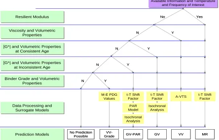
Chapter 7 presents the three ANN models that are ranked based on engineering judgment and statistical analysis of their predictability. From this prioritization, a decision tree structure has been developed for populating the |E*| of the LTPP layers (Figure 1.1). A user may follow this decision structure and determine the best model to use for the available input parameters. A key component to the prediction of moduli values is ensuring that the predicted values are rational and acceptable. To meet this criterion for the finalized ANN predictions, a set of quality control (QC) checks on both the input parameters and model predictions were performed. In total, seven different QC checks were developed, one for the inputs and six for the modulus predictions. These QC checks have been described in detail.
Executable software, “Artificial Neural Networks for Asphalt Concrete Dynamic Modulus Prediction” (ANNACAP), has been developed by the researchers at NCSU for this purpose1
. The software can be run for individual layers (manual mode) or all layers simultaneously (batch mode). A formal manual for the software is available (Kim et. al., 2009).
1 “ANNACAP” was developed by Maryam S. Sakhaeifar and B. Shane Underwood under the direction of Dr.
Chapter 1: Introduction
6
Resilient Modulus
Resilient Modulus
Viscosity and Volumetric Properties
Viscosity and Volumetric Properties No Yes Y N Y Prediction Models Prediction Models
Available Information and Temperature and Frequency of Interest Available Information and Temperature
and Frequency of Interest
|G*| and Volumetric Properties at Consistent Age
|G*| and Volumetric Properties
at Consistent Age
Data Processing and Surrogate Models
Data Processing and Surrogate Models t-T Shift Factor MR VV A-VTS GV-PAR No Prediction Possible t-T Shift Factor PAR Model Isochronal Analysis
Binder Grade and Volumetric Properties
Binder Grade and Volumetric
Properties N Y
M-E PDG Values
VV-Grade |G*| and Volumetric Properties
at Inconsistent Age
|G*| and Volumetric Properties
at Inconsistent Age
N Y GV t-T Shift Factor Isochronal Analysis N Resilient Modulus Resilient Modulus
Viscosity and Volumetric Properties
Viscosity and Volumetric Properties No Yes Y N Y Prediction Models Prediction Models
Available Information and Temperature and Frequency of Interest Available Information and Temperature
and Frequency of Interest
|G*| and Volumetric Properties at Consistent Age
|G*| and Volumetric Properties
at Consistent Age
Data Processing and Surrogate Models
Data Processing and Surrogate Models t-T Shift Factor MR VV A-VTS GV-PAR No Prediction Possible t-T Shift Factor PAR Model Isochronal Analysis t-T Shift Factor PAR Model Isochronal Analysis
Binder Grade and Volumetric Properties
Binder Grade and Volumetric
Properties N Y
M-E PDG Values
VV-Grade |G*| and Volumetric Properties
at Inconsistent Age
|G*| and Volumetric Properties
at Inconsistent Age
N Y GV t-T Shift Factor Isochronal Analysis t-T Shift Factor Isochronal Analysis N
Figure 1.1. Modulus prediction model decision tree.
Chapter 1: Introduction
7
predictions (i.e., an A grade), and 89, or 4.9 percent, of the total 1,806 layers have unreasonable predictions (i.e., an F grade). The remaining 306 layers, representing 17 percent of the 1,806 layers, have questionable predictions (i.e., a C grade). Thus, the total percentage of layers with a completely valid or questionable prediction is 51 percent. The quality grading system referenced is different than the standard Record Status definition used in the LTPP database. The research team established strict quality checks for these data to ensure that only the highest quality data were assigned an A grade. The data that did not achieve an A grade were not considered unusable data. All predictions are included in the database so that the user can determine the data that are suitable for their needs. In addition, the FHWA can revise the criteria used for the quality checks as deemed appropriate based on the opinions of their experts.
Chapter 8 presents outcomes from a research effort to develop new set of regression models for estimating the |E*| values if HMA mixtures. This set of models includes two closed-form models that can be used for the entire range of needed testing conditions and the remaining models are a series of five predictive models that are fully optimized and calibrated to be used in individual temperatures recommended in AASHTO TP-62 test protocol. In this chapter the performance of each model is thoroughly evaluated in different testing temperatures customarily used for measuring the |E*| values and by using a comprehensive set of independent database that were not used for calibrating any of these models.
Chapter 2: Literature Review
8
Chapter 2:
Literature Review
The dynamic modulus, |E*|, is a fundamental property that defines the stiffness characteristics of hot mix asphalt (HMA) mixtures as a function of loading rate and temperature. The significance of this material property is three-fold. First, it is one of the primary material property inputs in the Mechanistic-Empirical Pavement Design Guide (MEPDG) and software developed by NCHRP Project 1-37A (ARA, 2004). The MEPDG uses a mastercurve and time-temperature shift factors in its internal computations. In the MEPDG, the mastercurve is constructed using a hierarchical structure of inputs ranging from laboratory tests on HMA mixtures and binders to estimates based on properties of the HMA mixtures. Second, the |E*| is one of the primary HMA properties measured in the Superpave simple performance test protocol that complements the volumetric mix design. Third, the |E*| is one of the fundamental linear viscoelastic (LVE) material properties that can be used in advanced HMA and pavement models that are based on viscoelasticity.
In this part, the existing models used to estimate |E*| values and additional models that are developed based on the use of Artificial Neural Networks (ANNs) are evaluated. In addition to that the fundamental binder properties used in these models are described as well.
2.1.
PREDICTIVE MODELS
Chapter 2: Literature Review
9 Table 2.1. Predictive Relationships for |E*|.
Model # Model
1 Original Witczak Equation (NCHRP 1-37A)
2 Modified Witczak |G*| Equation (NCHRP 1-40D)
3 Hirsch Model
4 Law of Mixtures Parallel Model
5 ANN Model
6 MR-|E*| Model
2.1.1. Original Witczak Equation (NCHRP 1-37A)
Andrei et al. (1999) revised the original Witczak |E*| predictive equation based on data from 205 mixtures with 2750 data points. The revised equation is:
2
10 4
2
/ 3/8 /
log | * | 1.249937 0.02923 0.001767( ) 0.002841 0.05809
3.871977 0.0021 0.003958 0.000017( ) 0.00547 0.082208
1 exp( 0.603313 0.313351log 0.393532 log
a
beff
beff a
E p p p V
V p p p p
V V f
(2.1) where,
|E*| = dynamic modulus of HMA (105 psi);
p200 = percentage of aggregate passing #200 sieve;
p4 = percentage of aggregate retained in #4 sieve;
p3/8 = percentage of aggregate retained in 3/8 inch sieve;
p3/4 = percentage of aggregate retained in 3/4 inch sieve;
Va = percentage of air voids (by volume of mix);
Vbeff = percentage of effective asphalt content (by volume of mix);
f = loading frequency (Hz); and
Chapter 2: Literature Review
10
Witczak’s equation is based on nonlinear regression analysis using the Generalized Reduced Gradient optimization approach in Microsoft Excel’s Solver. This model incorporates mixture volumetric properties and aggregate gradation and is currently one of two options for Level 3 analysis using the NCHRP 1-37A MEPDG program. For the viscosity term in Equation (2.1), the program converts all Level 2 and 3 inputs into A-VTS values for the formulation of the |E*| mastercurve. Furthermore, Witczak’s model has an equation (not listed) to convert A-VTS coefficients from virgin or tank binders to RTFO- and PAV-aged binder values.
The limitations of Witczak’s equation, acknowledged by Bari et al. (2005), include reliance on other models to translate the currently used |G*| measurement into binder viscosity. It is also noted that because the model is based on regression analysis, extrapolation beyond the calibration database should be restricted. Bari et al. (2005) also mentions limited volumetric influence (precision) when the model is compared to the Shell Oil Model. Other researchers have also noted the need for improved sensitivity to volumetric properties, such as voids in mineral aggregate (VMA), voids filled with asphalt (VFA), asphalt content percentage (%AC) and air void percentage (%AV) (4).
2.1.2. Modified Witczak Equation Based on |G*| (NCHRP 1-40D)
Owing to the desire to include binder |G*|b in the predictive model, Witczak reformulated the
model in Equation (2.2) to include the binder variable directly. The updated model is:
2 2
4 4
0.0052
10 2
6.65 0.032 0.0027( ) 0.011 0.0001( )
log | * | 0.349 0.754 | * |
0.006 0.00014( ) 0.08 1.06
2.558 0.032 0.713 0.0124
b beff a beff a beff a beff a
p p p p
E G V
p p V
V V V V V V 2
/ 3 / 8 /
b
0.0001( ) 0.0098
1 exp( 0.7814 0.5785log | * |b 0.8834 log
p p p
G
Chapter 2: Literature Review
11 where,
|G*|b = dynamic shear modulus of asphalt binder (psi); and b = binder phase angle associated with |G*|b, (degrees).
As with the NCHRP 1-37A model, Equation (2.2) is based on a nonlinear regression analysis using 346 mixtures with 7400 total data points. The measured results of the unmodified binders have a better correlation with the model (R2 = 0.87) compared to those of the modified binders (R2 = 0.79) in arithmetic scale. In logarithmic scale, both binder types have R2 = 0.99. The binder phase angle is predicted using an empirical equation (R2 = 0.83). This equation is one of two options for Level 3 analysis in the most current MEPDG program. Because some of the mixtures in this database do not contain |G*|b data, the Cox-Mertz rule
using correction factors for the non-Newtonian behaviors, i.e., Equation (2.3), is used to calculate |G*|b from A-VTS values:
2
7.1542 0.4929 0.0211 ,
| * | 0.0051 (sin ) s s s
f f
b s f T b
G f
(2.3) ,
2 , 90 ( 7.3146 2.6162* ') *log( * )
(0.1124 0.2029* ') *log( * ) s s
b s f T
s f T
VTS f
VTS f
(2.4) 0.0527 0.0575
,
log log 0.9699 * 0.9668 * log
s
f T fs A fs VTS TR
, (2.5)
where,
fs = dynamic shear frequency;
b = binder phase angle predicted from Equation (2.4) (degrees);
fs,T = viscosity of asphalt binder at a particular loading frequency (fs) and
Chapter 2: Literature Review
12
2.1.3. Hirsch Model
Christensen et al. (2003) examined four different models based on the law of mixtures and chose the model that incorporates the binder modulus, VMA, and VFA, because it provides accurate results in the simplest form. The other, more complicated forms attempt to incorporate the modulus of the mastic or the film thickness, which are difficult parameters to measure. The suggested model for the |E*| estimation is as follows:
1 *
| * | 4, 200, 000 1 3 | * |
100 10, 000 1
100
4, 200, 000 3 | * |
c
m c b
b
P
VMA VFA VMA
E P G
VMA
VMA
G VFA
(2.6) 2
21 logPc) 55logPc
(2.7)
0.58
0.58 20 3 | * |
650 3 | * |
b c
b
G VFA VMA
P
G VFA VMA
(2.8)
where,
|E*|m = dynamic modulus of HMA in psi; Pc = the aggregate contact volume;
VMA = percentage of voids in mineral aggregate in compacted mixture; VFA = percentage of voids filled with asphalt in compacted mixture; and
= phase angle of HMA.
Chapter 2: Literature Review
13
parameter to account for the possible beneficial effects of modifiers (Al-Khateeb et al., 2006). Also, it must be noted that only 206 data points were used in determining the coefficients in the Hirsch model, compared to 2750 data points for the original Witczak model and 7400 data points for the modified Witczak model.
2.1.4. Law of Mixtures Parallel Model (Al-Khateeb Model)
Based on their findings from the Hirsch model, Al-Khateeb et al. (2006) suggest the following model:
0.66
0.66 | * |
90 10, 000 100
| * | 3 | * |
100 | * |
1,100 900
b
m g
b
G
VMA VMA
E G
G
VMA
(2.9)
where,
|G*|g = dynamic shear modulus of asphalt binder at the glassy state (assumed to be
145,000 psi).
Like the Hirsch model, this formulation is based on the law of mixtures for composite materials. In this model, the different material phases (aggregate, asphalt binder, and air) are considered to exist in parallel. This model, therefore, is a simpler interpretation of the Hirsch model. The researchers note that their model addresses one of the primary shortcomings of the Hirsch model, i.e., the Hirsch model’s inability to accurately predict the |E*| of the mixture at low frequencies and high temperatures.
Chapter 2: Literature Review
14
obtained from tests at higher than recommended strain amplitudes (200 µɛ versus the recommended maximum of 75-150 µɛ).
2.1.5. ANN Models
As part of this research study the Artificial Neural Network (ANN) technique was employed to develop new |E*| predictive models. The primary advantage of this approach over statistical regression is that the functional form of the relationship is not needed a priori. Considering that so many variables affect the |E*| values and their interactions, the ANN technique may capture complicated, nonlinear relationships between the |E*| and other mixture variables better than regression analysis.
The ANN technique is used in this research to develop several different models. The first is the ANN model that predicts the |E*| values using the input variables employed in the modified Witczak equation (i.e., binder dynamic modulus and phase angle, aggregate gradation, and volumetric properties of the HMA mixture). The effort to develop this ANN model is described later in Chapter 6. The ANN is also applied to backcalculate the |E*| values from the resilient modulus (MR). During the FHWA DTFH61-05-RA-00108 project,
the NCSU research team developed a mechanistic approach to compute the MR from the |E*|
of HMA (LaCroix et al., 2007). This approach has been verified successfully using measured data from mixtures with varying gradations and binder characteristics. The verified solutions were then applied to an available |E*| database to estimate the MR values corresponding to the
|E*| values. This database is used to develop an inverse algorithm based on the ANN technique that can predict the |E*| from the MR. The development and verification of the MR
Chapter 2: Literature Review
15
2.1.6. Regression Model
Regression analysis is any type of statistical techniques for modeling and analyzing several variables in order to find the relationship between a dependent variable and one or set of independent variables. Particularly, the regression analysis is helpful when the changes of dependent variable as a function of any one of the independent variables is desired while the others are held fixed. In this case the regression function is referred to the estimated target that is expressed as a function of the dependent variables (Lindley, 1987). This technique has been adopted in this research study to develop a new series of predictive models described in Chapter 8.
2.1.7. Summary of Input Variables
Table 2.2 presents the necessary input variables for each predictive relationship discussed previously. For models that utilize the |G*|b, predictions are only possible at the temperatures
and frequencies where |G*|b values are available. Having the |G*|b only at the conditions used
in Superpave™ testing is not sufficient for generating |E*| values over the range of conditions (-10° – 54°C) typically needed for mechanistic analysis. For example, if the user has the |G*|b only at 64°C and 10 rad/sec, then it is possible to predict the |E*| value only at
Chapter 2: Literature Review
16 Table 2.2. Model variables.
Variable Description Model No.
LTPP Data Availability 1 2 3 4 5 6 SPS1 GPS1
Mixture resilient modulus (MR) X Yes Yes
Binder shear modulus |G*|b X X X X Yes
2
No
Binder phase angle, b X X Yes No
Voids in mineral aggregate (%) X X Yes Yes4 Voids filled with asphalt (%) X Yes Yes4 Aggregate passing #200 sieve (%) X X X Yes Yes
Aggregate passing #4 sieve (%) X X X Yes Yes
Aggregate passing 3/8" sieve (%) X X X Yes Yes
Aggregate passing 3/4" sieve (%) X X X Yes Yes
Air voids (by Vmix) (%) X X X Yes Yes
Effective asphalt content (by Vtotal) (%) X X X Yes Yes 4
Loading frequency (Hz) X Yes No
Viscosities at temperatures of interest (A-VTS) X Yes3 Yes5
1 The in-service pavement sections are classified in the LTPP program as General Pavement Studies (GPS) and
Specific Pavement Studies (SPS).
2 |G*|
b was tested for SPS-9 sections only.
3 Penetration (77°F and 115°F), cone and plate viscometer (77°F), absolute viscosity (140°F), and
kinematic viscosity (275°F) data are available.
4
Reported by agency.
5 Ring and ball softening point, penetration (39.2°F and 77°F), absolute viscosity (140°F), and kinematic
viscosity (275°F) data are available (reported by agency).
A preliminary review of available information in the LTPP Materials database revealed that measured |G*|b data are only available for most of the SPS-9 projects and only at 10 rad/sec
at multiple temperatures. Even the available |G*|b data are measured from binders aged at
different levels (i.e., RTFO-aged versus PAV-aged). The lack of complete |G*|b data at
Chapter 2: Literature Review
17
model needs the binder time-temperature shift factor as well.) During the course of this project, the NCSU research team has developed empirical models that allow the estimation of the RTFO-aged |G*|b values at multiple temperatures and frequencies from the |G*|b values
obtained at a single frequency and multiple temperatures and aging levels (Kim et al., 2009).
2.2.
BINDER PROPERTIES
2.2.1. Shear Modulus
The behavior of asphalt is governed by both loading time and temperature. Therefore, the ideal test for expressing the LVE characteristics of the asphalt binder should consider both factors. The testing equipments that is customarily used and is capable of measuring the desired property is dynamic shear rheometer (DSR). Using DSR one can measure the rheological properties, shear modulus (|G*|) and phase angle () at intermediate to high temperatures. So, the dynamic shear modulus, |G*|, obtained based on DSR testing is known as the most popular material property to used for representing the asphalt binder component of asphalt concrete mixture (Al-Khateeb et al., 2006, Bari et al., 2005). Its popularity apparently stems from the fact that |G*| measurements are made as part of the existing purchase specification for asphalt binders, and it directly represents the LVE characteristics of the component material in asphalt concrete (the asphalt binder) that leads to the time dependence of the composite material.