2181
Learning to Progressively Recognize New Named Entities
with Sequence to Sequence Models
Lingzhen Chen
University of Trento Povo, Italy
Alessandro Moschitti∗
Amazon
Manhattan Beach, CA, USA
Abstract
In this paper, we propose to use a sequence to sequence model for Named Entity Recognition (NER) and we explore the effectiveness of such model in a progressive NER setting – a Transfer Learning (TL) setting. We train an initial model on source data and transfer it to a model that can recognize new NE categories in the target data during a subsequent step, when the source data is no longer available. Our solution consists in: (i) to reshape and re-parametrize the output layer of the first learned model to enable the recognition of new NEs; (ii) to leave the rest of the architecture unchanged, such that it is initialized with parameters transferred from the initial model; and (iii) to fine tune the network on the target data. Most importantly, we design a new NER approach based on sequence to sequence (Seq2Seq) models, which can intuitively work better in our progressive setting. We compare our approach with a Bidirectional LSTM, which is a strong neural NER model. Our experiments show that the Seq2Seq model performs very well on the standard NER setting and it is more robust in the progressive setting. Our approach can recognize previously unseen NE categories while preserving the knowledge of the seen data.
1 Introduction
Standard NER models are trained and tested on data with the same NE label set. In this paper, we explore a progressive setting, where (i) in the initial step, the model is trained on a datasetDSwith certain NE categories; and (ii) in the subsequent step, we further train the model on a dataset DT containing all categories fromDSalong with the new ones, without using the examples fromDSsince we assume they are no longer available. Our goal is to learn to recognize the new NE categories inDTwhile keeping the knowledge of previously seen categories.
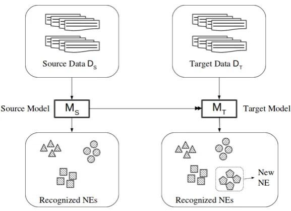
This study is motivated by the application of NER model in industry scenarios, where different com-panies may aim to recognize different types of NEs in the text. For example, users interested in finance would probably target entities such as companies or banks while other users interested in politics would target entities such as senators, bills, ministries, etc. Nevertheless, there are certain types of commonly-seen NE categories such as locations or dates that most users would like to recognize. These common NEs are typically provided with more available labeled data. Hence, methods that can utilize such data in new domains are rather useful. Additionally, the possibility to only use the models trained on such data is very important as it avoids the NER designer to deliver most training data to the user for adaptation in new domains. The setting above describes a TL problem, where the domain remains unchanged but the output space of the task changes: a graphical illustration of our progressive task is shown in Fig. 1.
Since the current state-of-the-art of NER is provided by neural models (Lample et al., 2016; Chiu and Nichols, 2016), we focus on them. In particular, we implement a baseline model with a bidirec-tional LSTM (BLSTM) as it is effective and does not require a heavy feature engineering for the task. BLSTM achieves competitive performance in comparisons with many other more complex state-of-the-art models, being much less complex. A drawback of such model is that, although its prediction takes the
∗
The main part of this work was carried out when the author was at the Unviversity of Trento.
Figure 1: Progressive NER task setting.
surrounding context of the input word into account, it does not explicitly model the dependencies of the label sequence. To better capture these dependencies, we propose the use of Seq2Seq models for NER.
We speculate that Seq2Seq models can be suitable for our NER task for the following reasons: (i) they can be used to translate from a source language (the word sequence) to the target language (the label sequence); and (ii) on the decoder side, the current prediction is able to take the previous prediction into account, by feeding the previous output together with current input. This is an important property to build NERs, since the output sequence has some dependency assumptions among them (e.g., B-LOC cannot be followed by I-PER). Intuitively, Seq2Seq models can separate the mapping from input to output into two steps: encoding the information from input to an intermediate hidden space, and decoding the intermediate information to the output space. When the output space changes, as in our experiment, the model ought to better leverage the use of previously learned knowledge since the encoding of the input is still similar to the previous task.
Our solution to the task consists in (i) modifying the output layer of the model by adding neurons for the new NE category; (ii) transferring the parameters in the source model trained on dataDSto the target model that is trained on dataDT; and (iii) fine-tuning the obtained network on the target data. As for the proposed Seq2Seq model, we modify the output layer only on the decoder side. We conduct extensive experiments on progressive NER, analyzing the performance of both models. Our main contribution is twofold, we show that the Seq2Seq model is: (i) effective for the NER task, and (ii) more robust in the progressive NER setting as it does not forget previously learned knowledge about seen NE categories.
2 Related Work
In this section, we report related works on current state-of-the-art models for standard NER task, as well as the related works in the Transfer Learning and Progressive Learning areas.
2.1 Neural Models for NER
pro-gressive NER since it is an effective model that does not require a heavy feature engineering for the task. The performance of BLSTM model are reported in different works (Lample et al., 2016; Chiu and Nichols, 2016): this also makes it easier for us to conduct a comprehensive comparison with other works.
2.2 Seq2Seq Models
Although not previously used for NER task, Seq2Seq models have seen a great success in various ap-plications, such as Neural Machine Translation by (Bahdanau et al., 2014; Luong et al., 2015), Speech Recognition (Lu et al., 2016; Zhang et al., 2017), Question Answering (Yin et al., 2016; Zhou et al., 2015) and so on. The idea of Seq2Seq model is to map a variable length source sequence to a fixed length vector representation by the encoder, and then remap it back to a variable length target sequence by the decoder. The Seq2Seq model was proposed by Cho et al. (2014) to learn phrase representations to be used in statistical Machine Translation. They reported empirical improvement of log-linear model performance while incorporating conditional probability of phrase pairs computed by the Seq2Seq model as additional features. Sutskever et al. (2014) also proposed a more general end-to-end approach to learn to map source sentences in one language into the translated sentences in the other.
To mitigate the bottleneck caused by mapping into a fixed-length vector, attention mechanism was proposed by Bahdanau et al. (2014). The attention mechanism works as a soft-alignment for the related parts in the source and target sequence. It is achieved by conditioning the prediction on a context vector that is calculated by the weighted sum of the encoder hidden states. Luong et al. (2015) further proposed global attention and local attention, to explore the effectiveness of different attention mechanisms. Our proposed model for NER is the same Seq2Seq architecture as proposed by Bahdanau et al. (2014), except that we use LSTM units for the encoder and decoder instead of simple RNN units. We also enforce an explicit alignment between the input word sequence and the output label sequence because the source and target sequences have a one-to-one mapping in the NER task.
2.3 Transfer Learning and Progressive Learning
Most machine learning methods assume the data for training and testing has the same feature space and distribution. TF is a technique that emerges to relax this assumption, allowing previously-learned knowledge to be used for a new task or in a new domain (Pan and Yang, 2010). Neural networks-based TL has proven to be very effective for image recognition (Donahue et al., 2014; Razavian et al., 2014). As for NLP, Mou et al. (2016) showed that TL can also be applied successfully on semantically equivalent NLP tasks. TL was applied on NER too, to transfer model and features on NER dataset with different NE entities (Qu et al., 2016; Kim et al., 2015).
Our learning paradigm falls in a more specific TL category – Progressive Learning. The Progressive Learning technique is adopted in multi-class classification by Venkatesan and Er (2016). They remodeled a network architecture (a single layer feed-forward network) by increasing the number of new neurons and interconnections while encountering unseen class labels in the dataset. The effectiveness of this technique is shown on several classic classification datasets. Our task is a sequence labeling task, where the independence assumption of output labels in a sequence does not hold. Hence, it cannot be treated as a set of classification tasks. We implement more sophisticated models and prove that the effectiveness of progressive learning techniques still holds.
3 Problem Formulation
In standard NER tasks, the model learns to maximize the conditional probabilityP(Y|X)whereX =
x1, x2, ..., xn(xi ∈ X)is the input word sequence andY =y1, y2, ..., yn(yi ∈ Y)is the output label
4 Models
We implemented (1) a BLSTM model, and (2) an attention-based Seq2Seq model for progressive NER. The input and output representation of both models is the expected to be the same.
4.1 Word & Character Embeddings
A word in the input sequence is represented by both its word-level and character-level embeddings. For the word-level representation, we use pretrained word embeddings to initialize an embedding lookup table to map the input wordx(represented by an integer index) to a vectorw.
A character-level representation is typically used because the NER task is sensitive to the morpho-logical traits of a word such as capitalization. They were shown to provide useful information for NER (Lample et al., 2016). We use a randomly initialized character embedding lookup table and then pass the embeddings to a character-level BLSTM (the details are described in Sec. 4.2) to obtain character level embeddingeforx.
The complete representation of the t-th word xt in the input sequence is the concatenation of its
word-level embeddingwtand character-level embeddinget.
4.2 Bidirectional LSTM
BLSTM model is composed of a forward LSTM (−LSTM) and a backward LSTM (−−−→ ←LSTM), which read−−−− the input sequence (represented as word vectors described in the previous subsection) in both left-to-right and reverse order. The output of the BLSTMhtis obtained by the concatenation of forward and backward output:ht= [
htcaptures the left and right context forxtand is then fed into a fully-connected layer. The output of
the fully connected layer ispt. The final prediction is obtained with a softmax over all possible tags as
P(yt=m|pt) =
eWo,mpt
P
m0∈MeWo,m0pt
,
where Woare parameters to be learned andM represents the set of all the possible output labels.
In the case of character-level BSLTM, the forward and backward LSTMs take the sequence of char-acter vectors[z1,z2, ...,zk]as input, wherekis the number of characters in a word. The final character
level embeddingetfor a word at timetis obtained by concatenating−→etand←et−.
4.3 Attention-based Encoder-Decoder
LSTM units are used in both encoder and decoder. On the encoder side, we use a BLSTM to capture the left and right context information of a word in the input sequence. The input to the encoder is the concatenation of word and character level embedding for each word, as the same as that for the BLSTM described above. The outputht = [
− → ht;
←−
ht]of the BLSTM at each time steptis later used for attention
calculation. On the decoder side, we use a single layer LSTM that generates label predictions step by step from the start to the end of the sentence. The last hidden state of the forward encoder RNN (−→ht) is used as
the initial decoder hidden state. At each decoding time step, the decoder hidden statestis calculated by st=σ(st−1,ct, yt−1,ht),wherest−1 is the previous decoder hidden state,ctis the context vector and
yt−1 is the previous prediction. ctis calculated as weighted sum of the encoder hidden state sequence
as follows: ct = T
X
j=1
αijhj,where T is the total length of a sentence. The weightαij is obtained by
applying a scoring function on the previous decoder hidden statest−1 and the aligned encoder hidden
Since we have a specific sequence to sequence task, where each element of the input at a positiont maps to an element of the output at the same positiont, we define an explicit alignment between encoder and decoder by feeding the encoder hidden statehtat timetto the decoder. We also restrict the decoder to output exactlyT label predictions by restricting the recurrent step of decoder LSTM asT. This ensures the one-to-one mapping between the input words and the output labels. The final prediction ofytis made
by passingstto a fully-connected layer and then applying a softmax function over the output of this layer
(the same as described in Sec. 4.2).
4.4 Progressive Adaption
Our proposed method for progressive NER is through pre-training a source model, transferring param-eters to the target model and then fine-tuning such model. In the initial step, the model is trained on labeled source data until the optimal parametersθˆSare obtained and saved. θˆSinclude the parameters regarding the output layerθˆS
outputand those regarding all the other layersθˆ−Soutput.
To recognize the new NE categories, the major modification is made on the fully-connected layer after the BLSTM, i.e., the output layer of the network. In the BLSTM architecture, the fully-connected layer maps the outputhof BLSTM to a vectorpof sizenC. nis a factor depending on the tagging format of the dataset (e.g., n = 4if the dataset is in the BIOES format1, since for each NE category, there would be 4 output labelsB-NE,I-NE,E-NE andS-NE). To recognize the target NEs, we build the same model architecture for all layers before the output layer and initialize all their parameters by θˆ−Soutput
obtained in the initial step. We extend the output layer withnE nodes, whereE is the number of new NE categories. These are initialized with weights drawn from the random distributionX ∼ N(µ, σ2), whereµandσare the mean and standard deviation of the pre-trained weights in the same layer. 2 This way, the associated weight matrix of the fully-connected layerWso also updates from the original shape nC×pto a new matrixWso0 of shape(nC+nE)×p. Note thatθˆSoutputandθˆ−Soutputare essentially the weights in the matrixWso andWs−o. The new model parameters are updated in the same way as in the
initial step.
5 Experiments
5.1 Data
We used the CONLL 2003 NER dataset3 by modifying it to suit our experiment settings. The original dataset includes news articles with four types of named entities – organization, person, location and miscellaneous (represented byORG,PER,LOC, andMISC, respectively). TheOlabel indicates tokens that do not belong to any of these four named entities. The entity labels are annotated in BIOES format. For the purpose of our experiment, we shuffle and divide the training set into 80%/20% partitions as DSandDTfor the initial and the subsequent steps, as we assume that the size of the target data would be less than that of the source data. The validation and the test sets are the same in both steps in terms of the sentence instances, but different in label annotation. In particular, we create four datasets by (i) selecting one of the four categories as the new NE category to be recognized in the subsequent step; and (ii) substituting the labels of such category withO(not an entity) inDtrainS,DvalidS andDtestS. For example, when we useLOCas the new NE, we replace all theLOClabel annotations withO, where they appear inDtrainS,DvalidSandDtestS. Instead, inDtrainT,DvalidT andDtestT, we keepLOC label annotation as is. A summary of label statistics for each case is shown in Table 1.
Apart from dividing the dataset into two components DS and DT, we do not perform any specific pre-processing of the dataset, except for replacing all digits with 0 to reduce the size of the vocabulary.
1
The BIOES format (short for Begin, Inside, Outside, End and Single) is a common tagging format for tagging tokens. 2We initialize the weights using the approach producing the higher accuracy on the validation set. Our initizialization
options are (i) set all parameters to zeros; (ii) using the random distributionX ∼ N(µ, σ2), whereµ= 0.0andσ = 1.0; and (iii) using the random distributionX ∼ N(µ, σ2), whereµandσare the mean and standard deviation of the pre-trained weights in the same layer.
Set LOC PER ORG MISC
Table 1: Number of labels after customizing CONLL dataset for the progressive NER experiments. Init. and Sub. represent the initial and the subsequent steps, respectively.
Parameter Value Range
batch size 128 [16, 32, 64, 128, 256] clip value 5.0 ([5.0, 50.0], 1.0) char hidden size 25 ([5, 25], 5) word hidden size 128 [64, 72, 128, 256, 512]
dropout rate 0.5 ([0.1, 0.8], 0.1) word hidden size 72 [64, 72, 128, 256, 512]
dropout rate 0.4 ([0.1, 0.8], 0.1) learning rate 0.02 ([0.0025, 0.01], 0.0025)
(b) Seq2Seq model
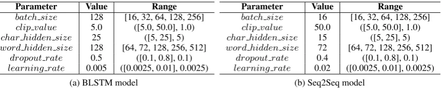
Table 2: Value range and final value of hyperparameters for the BLSTM and the Seq2Seq models.
5.2 Models
We use 100 dimension GLOVE pretrained embedding4 to initialize the word embedding lookup table. Since we do not lowercase the tokens in the input sequences, the words without direct mappings to the pretrained word embeddings are initialized as their lowercase counterparts, if found in the pretrained word embeddings. We replace the infrequent words, i.e., appearing less than two in the training set or in the test set, with<UNK>. The word embedding for<UNK>is randomly initialized by drawing from a uniform distribution between[−0.25,0.25].
We perform hyperparameter optimization by a Random Search (Bergstra and Bengio, 2012) on differ-ent intervals for each hyperparameter for both models, including the size for the character and word level embeddings of the BLSTMs, the batch size, the learning rate, the dropout rate and the maximum value for gradient clipping. Tab. 2 shows the intervals and the final values for each hyperparameter, where the final values are the ones giving the best performance on the validation set (DvalidS) in each experiment setting.
5.3 Training
Init. Sub. Rand.
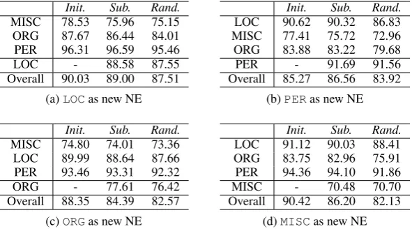
Table 3: Test F1 of the BLSTM model on each category.
Init. Sub. Rand.
Table 4: Test F1 of the Seq2Seq model on each category.
5.4 Results
Our baseline BLSTM model performs in-line with the BLSTM models reported by Lample et al. (2016) or by Chiu and Nichols (2016). We obtained an overall F1 score of 89.74 on traditional setting of NER. The Seq2Seq model outperformed the baseline model by 1.24 points in F1, reaching 90.98. The latter is comparable to some of the state-of-the-art results reported on the CONLL dataset.
5.4.1 Performance on Source Data
The performance of the BLSTM and Seq2Seq models in our progressive learning setting is shown in tables 3 and 4, respectively. Sub-level tables (a), (b), (c) and (d) report the test F1 in different experiment settings – recognizing different target new NE in the subsequent step. Init. indicates the F1 scores in the initial step, whileSub. indicates the scores in the subsequent step. Rand. reports the test F1 scores obtained by the same model architecture but with randomly initialized parameters and trained with all the target data in the subsequent step.
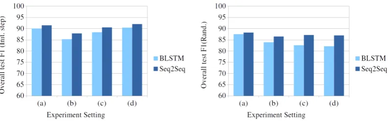
The training in the initial step and for the model with randomly initialized parameter in the subsequent step can be seen as a standard NER task. We further report a comparison of the performance of both models in the initial step as well as with the randomly initialized parameters in Figure 2. We can see that the Seq2Seq model outperforms the BLSTM model in all experiment settings. This supports our argument that the Seq2Seq model can be a better approach for the NER task than BLSTM due to its ability to exploit the previous predicted labels.
4
http://nlp.stanford.edu/data/glove.6B.zip
(a) Overall test F1 in the initial step (b) Overall test F1 in the subsequent step (Rand.)
Figure 2: A comparison of between the BLSTM and Seq2Seq models on standard NER task.
5.4.2 Transferred Parameters vs. Randomly Initialized Parameters
By construction, there is always a label disagreement between the data of the initial and of the subsequent steps for the new NE, as it is annotated asOin the data for the initial step. We can derive some interesting observations from the comparison between the F1 of the model using randomly initialized parameters (ColumnRand. in each table) and the F1 of the model using transferred parameters in the subsequent step (Column Sub. in each table). In almost all cases, using transferred parameters produces better performance, by around 2 to 3 points in F1. In terms of the target new NE category, the models using transferred parameters are able to perform better than the models with only randomly-initialized param-eters. This is because we allow the transferred parameters to be updated together with the other model parameters in the subsequent step. Such approach can recover from the adverse knowledge learned in the initial step with regard to treating the target new label asO. The only exception is when usingMISC as target new NE. The F1 obtained by randomly initialized parameters for both BLSTM and Seq2Seq model is higher than the one obtained by the models using transferred parameters. This may be explained by the fact that theMISCcategory is a collection of NEs that do not fit into other categories. Thus, the context of such NEs may vary a lot from one to another, making the recovery from the previously-learned adverse knowledge on this NE category more challenging, e.g., its new context and information in the subsequent step are sparser.
We allow a maximum of 200 epochs in the subsequent step while forcing the training to stop when the F1 score on the validation set does not improve for more than 30 epochs. Even if we increase the training epochs to 60 for the model using randomly initialized parameters, transferred parameters still perform better. We also observed that the model with transferred parameters converges faster during the subsequent training, in around 20 epochs. This suggests that our progressive learning technique enables the models to more accurately predict the new categories and in a shorter time. That is, the transferred parameters not only help the model to reach a superior performance, but also provide a better initialization for the model to converge faster.
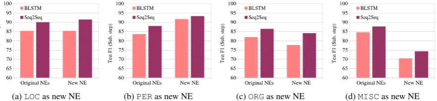
5.4.3 Original NE Classes vs. New Target NE Class
The improvement or decrease of the F1 for the original NE categories is an indicator of how well the model is able to preserve the learned knowledge transferred from the initial step. In Table 5, we report the difference of test F1 between the initial and the subsequent steps, for each of the original NE categories, using the BLSTM and Seq2Seq models. In this table, lower value means a lower loss in the F1 score, i.e., the model is better in preserving the performance on the NE categories that are seen in the initial step. In almost all cases, the Seq2Seq model suffers less degradation in F1. In some cases, the Seq2Seq model is able to further learn from the subsequent data and achieve better performance on these original NE categories. For example, when using PER as the new NE category, the Seq2Seq model is able to improve the performance onLOCandMISC, while the BLSTM model decreases its F1.
LOC as new NE PER as new NE ORG as new NE MISC as new NE
BLSTM Seq2Seq BLSTM Seq2Seq BLSTM Seq2Seq BLSTM Seq2Seq
MISC 2.51 2.03 1.69 -0.07 0.79 -0.88 -
-ORG 1.23 1.07 0.66 0.71 - - 0.79 0.79
PER -0.28 -0.07 - - 0.15 0.12 0.26 0.11
LOC - - 0.30 -0.09 1.35 -0.03 1.09 0.17
Table 5: Difference of the test F1 score from the initial step to the subsequent step (lower value is better, while a negative value means that the model is able to further improve).
BLSTM Seq2Seq
LOC 88.58 91.33
PER 91.96 93.30
ORG 77.61 84.11
MISC 70.48 74.28
Table 6: Test F1 on the new target NE in the subsequent step.
(a)LOCas new NE (b)PERas new NE (c)ORGas new NE (d)MISCas new NE
Figure 3: Test F1 scores obtained on the original NEs and the target new NE by the BLSTM and the Seq2Seq model.
Table 6. As it is evident from the table, in all cases, the Seq2Seq model produces better test F1 scores by 2 to 3 points at least. In the case ofORGlabel, the performance of the Seq2Seq model surpasses that of the BLSTM model by nearly 7 points. By comparing both the performance on the original labels and on the target new label, as shown in Figure 3, we see that the performance of Seq2Seq model is better than the baseline BLSTM in both the original and the new NE classes. It can be concluded that Seq2Seq model is more robust in the subsequent step regarding recognizing the new target NE category while it does not degrade the performance of the original NE categories.
6 Conclusions
In this work, we propose to use attention-based Seq2Seq models for both standard NER task as well as the progressive NER task, which is a more practical scenario of industry level applications of NER. We argue that the Seq2Seq model is suitable for both settings. Our experimental results support our claim as the Seq2Seq model outperforms BLSTM in both standard and progressive NER settings. Further analyses show that the Seq2Seq model is better in both preserving the knowledge learned from the source data, and in learning the new knowledge from the target data. We also demonstrated the effectiveness of the proposed progressive learning technique in the NER task. In future work, we would like to experiment with other datasets as well as extend our methods to target data that is only annotated with the new NE category. It would be also interesting to apply our model and technique to other areas such as domain adaptation or few-shot learning.
Acknowledgements
References
Dzmitry Bahdanau, Kyunghyun Cho, and Yoshua Bengio. 2014. Neural machine translation by jointly learning to align and translate. CoRR, abs/1409.0473.
James Bergstra and Yoshua Bengio. 2012. Random search for hyper-parameter optimization.Journal of Machine Learning Research, 13:281–305.
Xavier Carreras, Llu´ıs M`arquez, and Llu´ıs Padr´o. 2003. Learning a perceptron-based named entity chunker via online recognition feedback. InProceedings of the Seventh Conference on Natural Language Learning, CoNLL 2003, Held in cooperation with HLT-NAACL 2003, Edmonton, Canada, May 31 - June 1, 2003, pages 156–159.
Hai Leong Chieu and Hwee Tou Ng. 2003. Named entity recognition with a maximum entropy approach. In
Proceedings of the Seventh Conference on Natural Language Learning, CoNLL 2003, Held in cooperation with HLT-NAACL 2003, Edmonton, Canada, May 31 - June 1, 2003, pages 160–163.
Jason P. C. Chiu and Eric Nichols. 2016. Named entity recognition with bidirectional lstm-cnns. TACL, 4:357– 370.
Kyunghyun Cho, Bart van Merrienboer, C¸ aglar G¨ulc¸ehre, Dzmitry Bahdanau, Fethi Bougares, Holger Schwenk, and Yoshua Bengio. 2014. Learning phrase representations using RNN encoder-decoder for statistical machine translation. InProceedings of the 2014 Conference on Empirical Methods in Natural Language Processing, EMNLP 2014, October 25-29, 2014, Doha, Qatar, A meeting of SIGDAT, a Special Interest Group of the ACL, pages 1724–1734.
Jeff Donahue, Yangqing Jia, Oriol Vinyals, Judy Hoffman, Ning Zhang, Eric Tzeng, and Trevor Darrell. 2014. Decaf: A deep convolutional activation feature for generic visual recognition. In Proceedings of the 31th International Conference on Machine Learning, ICML 2014, Beijing, China, 21-26 June 2014, pages 647–655.
Radu Florian, Abraham Ittycheriah, Hongyan Jing, and Tong Zhang. 2003. Named entity recognition through classifier combination. InProceedings of the Seventh Conference on Natural Language Learning, CoNLL 2003, Held in cooperation with HLT-NAACL 2003, Edmonton, Canada, May 31 - June 1, 2003, pages 168–171.
Young-Bum Kim, Karl Stratos, Ruhi Sarikaya, and Minwoo Jeong. 2015. New transfer learning techniques for disparate label sets. InProceedings of the 53rd Annual Meeting of the Association for Computational Linguistics and the 7th International Joint Conference on Natural Language Processing of the Asian Federation of Natural Language Processing, ACL 2015, July 26-31, 2015, Beijing, China, Volume 1: Long Papers, pages 473–482.
Guillaume Lample, Miguel Ballesteros, Sandeep Subramanian, Kazuya Kawakami, and Chris Dyer. 2016. Neural architectures for named entity recognition. InNAACL HLT 2016, The 2016 Conference of the North Amer-ican Chapter of the Association for Computational Linguistics: Human Language Technologies, San Diego California, USA, June 12-17, 2016, pages 260–270.
Liang Lu, Xingxing Zhang, and Steve Renals. 2016. On training the recurrent neural network encoder-decoder for large vocabulary end-to-end speech recognition. In2016 IEEE International Conference on Acoustics, Speech and Signal Processing, ICASSP 2016, Shanghai, China, March 20-25, 2016, pages 5060–5064.
Thang Luong, Hieu Pham, and Christopher D. Manning. 2015. Effective approaches to attention-based neu-ral machine translation. InProceedings of the 2015 Conference on Empirical Methods in Natural Language Processing, EMNLP 2015, Lisbon, Portugal, September 17-21, 2015, pages 1412–1421.
Lili Mou, Zhao Meng, Rui Yan, Ge Li, Yan Xu, Lu Zhang, and Zhi Jin. 2016. How transferable are neural networks in NLP applications? In Proceedings of the 2016 Conference on Empirical Methods in Natural Language Processing, EMNLP 2016, Austin, Texas, USA, November 1-4, 2016, pages 479–489.
Sinno Jialin Pan and Qiang Yang. 2010. A survey on transfer learning. IEEE Trans. Knowl. Data Eng., 22(10):1345–1359.
Adam Paszke, Sam Gross, Soumith Chintala, Gregory Chanan, Edward Yang, Zachary DeVito, Zeming Lin, Alban Desmaison, Luca Antiga, and Adam Lerer. 2017. Automatic differentiation in pytorch.
Lizhen Qu, Gabriela Ferraro, Liyuan Zhou, Weiwei Hou, and Timothy Baldwin. 2016. Named entity recognition for novel types by transfer learning. InProceedings of the 2016 Conference on Empirical Methods in Natural Language Processing, EMNLP 2016, Austin, Texas, USA, November 1-4, 2016, pages 899–905.
Ilya Sutskever, Oriol Vinyals, and Quoc V. Le. 2014. Sequence to sequence learning with neural networks. In
Advances in Neural Information Processing Systems 27: Annual Conference on Neural Information Processing Systems 2014, December 8-13 2014, Montreal, Quebec, Canada, pages 3104–3112.
Rajasekar Venkatesan and Meng Joo Er. 2016. A novel progressive learning technique for multi-class classifica-tion. Neurocomputing, 207:310–321.
Jun Yin, Xin Jiang, Zhengdong Lu, Lifeng Shang, Hang Li, and Xiaoming Li. 2016. Neural generative question answering. InProceedings of the Twenty-Fifth International Joint Conference on Artificial Intelligence, IJCAI 2016, New York, NY, USA, 9-15 July 2016, pages 2972–2978.
Yu Zhang, William Chan, and Navdeep Jaitly. 2017. Very deep convolutional networks for end-to-end speech recognition. In 2017 IEEE International Conference on Acoustics, Speech and Signal Processing, ICASSP 2017, New Orleans, LA, USA, March 5-9, 2017, pages 4845–4849.