A Sensitivity Analysis of (and Practitioners’ Guide to) Convolutional
Neural Networks for Sentence Classification
Ye Zhang
Dept. of Computer Science University of Texas at Austin
Byron C. Wallace
College of Computer and Information Science Northeastern University
Abstract
Convolutional Neural Networks (CNNs) have recently achieved remarkably strong performance on the practically important task of sentence classification (Kim,2014;
Kalchbrenner et al., 2014; Johnson and
Zhang, 2014; Zhang et al., 2016).
How-ever, these models require practitioners to specify an exact model architecture and set accompanying hyperparameters, includ-ing the filter region size, regularization pa-rameters, and so on. It is currently un-known how sensitive model performance is to changes in these configurations for the task of sentence classification. We thus conduct a sensitivity analysis of one-layer CNNs to explore the effect of architecture components on model performance; our aim is to distinguish between important and comparatively inconsequential design decisions for sentence classification. We focus on one-layer CNNs (to the exclu-sion of more complex models) due to their comparative simplicity and strong empiri-cal performance, which makes it a modern standard baseline method akin to Support Vector Machine (SVMs) and logistic re-gression. We derive practical advice from our extensive empirical results for those interested in getting the most out of CNNs for sentence classification in real world settings.
1 Introduction
Convolutional Neural Networks (CNNs) have re-cently been shown to achieve impressive results on the practically important task of sentence cate-gorization (Kim,2014;Kalchbrenner et al.,2014;
Wang et al., 2015; Goldberg, 2015; Iyyer et al.,
2015;Zhang et al.,2016,2017). CNNs can
cap-italize on distributed representations of words by first converting the tokens comprising each sen-tence into a vector, forming a matrix to be used as input (e.g., see Fig.1). The models need not be complex to realize strong results: Kim (2014), for example, proposed a simple one-layer CNN that achieved state-of-the-art (or comparable) results across several datasets. The very strong results achieved with this comparatively simple CNN ar-chitecture suggest that it may serve as a drop-in replacement for well-established baseline models, such as SVM (Joachims,1998) or logistic regres-sion. While more complex deep learning models for text classification will undoubtedly continue to be developed, those deploying such technolo-gies in practice will likely be attracted to simpler variants, which afford fast training and prediction times.
Unfortunately, a downside to CNN-based mod-els – even simple ones – is that they require prac-titioners to specify the exact model architecture to be used and to set the accompanying hyperpa-rameters. In practice, tuning all of these hyper-parameters is simply not feasible, especially be-cause parameter estimation is computationally in-tensive. Emerging research has begun to explore hyperparameter optimization methods, including random search (Bengio,2012), and Bayesian op-timization (Yogatama and Smith, 2015; Bergstra
et al.,2013). However, these sophisticated search
methods still require knowing which hyperparam-eters are worth exploring to begin with (and rea-sonable ranges for each).
In this work our aim is to identify empirically the settings that practitioners should expend effort tuning, and those that are either inconsequential with respect to performance or that seem to have a ‘best’ setting independent of the specific dataset, and provide a reasonable range for each
rameter. We take inspiration from previous empir-ical analyses of neural models due to Coates et al. (2011) and Breuel (2015), which investigated fac-tors in unsupervised feature learning and hyperpa-rameter settings for Stochastic Gradient Descent (SGD), respectively. Here we report the results of a large number of experiments exploring differ-ent configurations of CNNs run over nine sdiffer-entence classification datasets. Most previous work in this area reports only mean accuracies calculated via cross-validation. But there is substantial variance in the performance of CNNs, even on the same foldsand with model configuration held constant. Therefore, in our experiments we perform replica-tions of cross-validation and report accuracy/Area Under Curve (AUC) score means and ranges over these.
2 Background and Preliminaries
Deep and neural learning methods are now well established in machine learning (LeCun et al.,
2015; Bengio, 2009). They have been
espe-cially successful for image and speech process-ing tasks. More recently, such methods have be-gun to overtake traditional sparse, linear models for NLP (Goldberg, 2015; Bengio et al., 2003;
Mikolov et al.,2013;Collobert and Weston,2008;
Collobert et al.,2011;Kalchbrenner et al.,2014;
Socher et al.,2013).
Recently, word embeddings have been ex-ploited for sentence classification using CNN ar-chitectures. Kalchbrenner (2014) proposed a CNN architecture with multiple convolution lay-ers, positing latent, dense and low-dimensional word vectors (initialized to random values) as in-puts. Kim (2014) defined a one-layer CNN archi-tecture that performed comparably. This model uses pre-trained word vectors as inputs, which may be treated asstatic ornon-static. In the for-mer approach, word vectors are treated as fixed inputs, while in the latter they are ‘tuned’ for a specific task. Elsewhere, Johnson and Zhang (2014) proposed a similar model, but swapped in high dimensional ‘one-hot’ vector representations of words as CNN inputs. Their focus was on clas-sification of longer texts, rather than sentences (but of course the model can be used for sentence clas-sification).
The relative simplicity of Kim’s architecture – which is largely the same as that proposed by Johnson and Zhang (2014), modulo the word
vec-tors – coupled with observed strong empirical per-formance makes this a strong contender to sup-plant existing text classification baselines such as SVM and logistic regression. But in practice one is faced with making several model architecture decisions and setting various hyperparameters. At present, very little empirical data is available to guide such decisions; addressing this gap is our aim here.
2.1 CNN Architecture
We begin with a tokenized sentence which we then convert to a sentence matrix, the rows of which are word vector representations of each to-ken. These might be, e.g., outputs from trained word2vec (Mikolov et al., 2013) or GloVe (
Pen-nington et al., 2014) models. We denote the
di-mensionality of the word vectors by d. If the length of a given sentence is s, then the dimen-sionality of the sentence matrix iss×d. Suppose that there is a filter matrixwwith region sizeh;w
will containh·dparameters to be estimated. We denote the sentence matrix byA∈Rs×d, and use A[i:j]to represent the sub-matrix ofAfrom row
ito rowj. The output sequenceo ∈ Rs−h+1 of
the convolution operator is obtained by repeatedly applying the filter on sub-matrices ofA:
oi =w·A[i:i+h−1], (1)
wherei = 1. . . s−h+ 1, and·is the dot prod-uct between the sub-matrix and the filter (a sum over element-wise multiplications). We add a bias termb ∈ R and an activation functionf to each
oi, inducing thefeature mapc ∈ Rs−h+1 for this
filter:
ci =f(oi+b). (2)
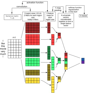
et al.,2012) as a means of regularization. This en-tails randomly setting values in the weight vector to 0. One may also impose anl2norm constraint, i.e., linearly scale thel2 norm of the vector to a pre-specified threshold when it exceeds this. Fig.
1 provides a schematic illustrating the model ar-chitecture just described. The training objective to be minimized is the categorical cross-entropy loss. The parameters to be estimated include the weight vector(s) of the filter(s), the bias term in the acti-vation function, and the weight vector of the soft-max function. In the ‘non-static’ approach, one also tunes the word vectors. Optimization is per-formed using SGD and back-propagation (
Rumel-hart et al.,1988).
3 Datasets
We use nine sentence classification datasets in all; seven of which were also used by Kim (2014). Briefly, these are summarized as follows. (1) MR: sentence polarity dataset from (Pang and Lee,2005). (2)SST-1: Stanford Sentiment Tree-bank (Socher et al., 2013). To make input repre-sentations consistent across tasks, we only train and test on sentences, in contrast to the use in (Kim,2014), wherein models were trained on both phrases and sentences. (3)SST-2: Derived from SST-1, but pared to only two classes. We again only train and test models on sentences, excluding phrases. (4)Subj: Subjectivity dataset (Pang and Lee, 2005). (5) TREC: Question classification dataset (Li and Roth, 2002). (6) CR: Customer review dataset (Hu and Liu, 2004). (7) MPQA: Opinion polarity dataset (Wiebe et al.,2005). Ad-ditionally, we use (8) Opi: Opinosis Dataset, which comprises sentences extracted from user re-views on a given topic, e.g. “sound quality of ipod nano”. There are 51 such topics and each topic contains approximately 100 sentences (Ganesan
et al.,2010). (9)Irony(Wallace et al.,2014): this
contains 16,006 sentences from reddit labeled as ironic (or not). The dataset is imbalanced (rela-tively few sentences are ironic). Thus before train-ing, we under-sampled negative instances to make classes sizes equal.1 For this dataset we report the Area Under Curve (AUC), rather than accuracy, because it is imbalanced.
1Empirically, under-sampling outperformed over-sampling in mitigating imbalance, see also Wallace (2011).
4 Baseline Models 4.1 Baseline Configuration
We give a baseline CNN configuration described in Table1. We argue that it is critical to assess the variance due strictly to the parameter estimation procedure. Most prior work, unfortunately, has not reported such variance, despite a highly stochastic learning procedure. This variance is attributable to estimation via SGD, random dropout, and random weight parameter initialization.
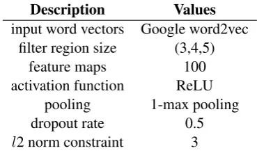
Description Values
input word vectors Google word2vec filter region size (3,4,5)
feature maps 100
activation function ReLU
pooling 1-max pooling
dropout rate 0.5
l2 norm constraint 3
Table 1: Baseline configuration. ‘feature maps’ refers to the number of feature maps for each filter region size. ‘ReLU’ refers torectified linear unit
(Maas et al., 2013), a commonly used activation
function in CNNs.
Then we consider the effect of different archi-tecture decisions and hyperparameter settings. To this end, we hold all other settings constant (as per Table1) and vary only the component of interest. For every configuration that we consider, we repli-cate the experiment 10 times, where each replica-tion constitutes a run of 10-fold CV. We report av-erage CV means and associated ranges achieved over the replicated CV runs.
4.2 Effect of input word vectors
A nice property of sentence classification models that start with distributed representations of words as inputs is the flexibility such architectures afford to swap in different pre-trained word vectors dur-ing model initialization. Therefore, we first ex-plore the sensitivity of CNNs for sentence classi-fication with respect to the input representations used. Specifically, we replaced word2vec with GloVe representations. Google word2vec uses a local context window model trained on 100 billion words from Google News (Mikolov et al.,2013), while GloVe is a model based on global word-word co-occurrence statistics (Pennington et al.,
cor-I like this movie
very much
!
2 feature maps for each region size
6 univariate vectors concatenated together to form a
single feature vector
Sentence matrix 7× 5
3 region sizes: (2,3,4) 2 filters for each region
size totally 6 filters convolution
activation function
1-max pooling
2 classes
softmax function regularization in this layer
d=5
Figure 1: Illustration of a CNN architecture for sentence classification. We depict three filter region sizes: 2, 3 and 4, each of which has 2 filters. Filters perform convolutions on the sentence matrix and generate (variable-length) feature maps; 1-max pooling is performed over each map, i.e., the largest number from each feature map is recorded. Thus a univariate feature vector is generated from all six maps, and these 6 features are concatenated to form a feature vector for the penultimate layer. The final softmax layer then receives this feature vector as input and uses it to classify the sentence; here we assume binary classification and hence depict two possible output states.
pus of 840 billion tokens of web data. For both word2vec and GloVe we induce 300-dimensional word vectors. We report results achieved using GloVe representations in Table 2. Here we only report non-static GloVe results (which uniformely outperformed the static variant).
We also experimented with concatenating word2vec and GloVe representations, thus cre-ating 600-dimensional word vectors to be used as input to the CNN. Pre-trained vectors may not always be available for specific words (ei-ther in word2vec or GloVe, or both); in such cases, we randomly initialized the correspond-ing sub-vectors. Results are reported in the fi-nal column of Table 2. The relative performance
achieved using GloVe versus word2vec depends on the dataset, and, unfortunately, simply concate-nating these representations does necessarily seem helpful. For how to better utilize multiple sets of embeddings, we refer to (Zhang et al.,2016).
con-Dataset Non-static word2vec-CNN Non-static GloVe-CNN Non-static GloVe+word2vec CNN
MR 81.24 (80.69, 81.56) 81.03 (80.68,81.48) 81.02 (80.75,81.32) SST-1 47.08 (46.42,48.01) 45.65 (45.09,45.94) 45.98 (45.49,46.65) SST-2 85.49 (85.03, 85.90) 85.22 (85.04,85.48) 85.45 (85.03,85.82) Subj 93.20 (92.97, 93.45) 93.64 (93.51,93.77) 93.66 (93.39,93.87) TREC 91.54 (91.15, 91.92) 90.38 (90.19,90.59) 91.37 (91.13,91.62) CR 83.92 (82.95, 84.56) 84.33 (84.00,84.67) 84.65 (84.21,84.96) MPQA 89.32 (88.84, 89.73) 89.57 (89.31,89.78) 89.55 (89.22,89.88) Opi 64.93 (64.23,65.58) 65.68 (65.29,66.19) 65.65 (65.15,65.98) Irony 67.07 (65.60,69.00) 67.20 (66.45,67.96) 67.11 (66.66,68.50)
Table 2: Performance using non-static word2vec-CNN, non-static GloVe-CNN, and non-static GloVe+word2vec CNN, respectively. Each cell reports the mean (min, max) of summary performance measures calculated over multiple runs of 10-fold cross-validation. We will use this format for all tables involving replications
figuration, and the one-hot vector is fixed during training. Compared to using embeddings as in-put to the CNN, we found the one-hot approach to perform poorly for sentence classification tasks. We believe that one-hot CNN may not be suit-able for sentence classification, likely due to spar-sity: the sentences are perhaps too brief to provide enough information for this high-dimensional en-coding. Alternative one-hot architectures (
John-son and Zhang,2015) might be more appropriate
for this scenario.
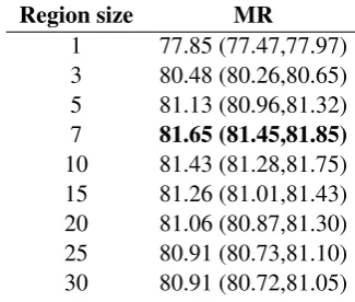
4.3 Effect of filter region size
Region size MR
1 77.85 (77.47,77.97) 3 80.48 (80.26,80.65) 5 81.13 (80.96,81.32) 7 81.65 (81.45,81.85) 10 81.43 (81.28,81.75) 15 81.26 (81.01,81.43) 20 81.06 (80.87,81.30) 25 80.91 (80.73,81.10) 30 80.91 (80.72,81.05)
Table 3: Effect of single filter region size. Due to space constraints, we report results for only one dataset here, but these are generally illustrative.
We first explore the effect of filter region size when using only one region size, and we set the number of feature maps for this region size to 100 (as in the baseline configuration). We consider re-gion sizes of 1, 3, 5, 7, 10, 15, 20, 25 and 30, and record the means and ranges over 10 replications of 10-fold CV for each. We report results in Ta-ble3and Fig. 2. Because we are only interested in the trend of the accuracy as we alter the region size (rather than the absolute performance on each
1 3 5 7 10 15 20 25 30 Filter region size
6 5 4 3 2 1 0 1 2
Change in accuracy (%)
MR SST-1 SST-2 Subj TREC CR MPQA Opi Opi
Figure 2: Effect of the region size (using only one).
task), we show only the percent change in accu-racy (AUC for Irony) from an arbitrary baseline point (here, a region size of 3).
different filter region sizes close to this optimal range, and compared this to approaches that use region sizes outside of this range. From Table
5, one can see that using (5,6,7),and (7,8,9) and (6,7,8,9) – sets near the best single region size – produce the best results. The difference is espe-cially pronounced when comparing to the base-line setting of (3,4,5). Note that even only using a single good filter region size (here, 7) results in better performance than combining different sizes (3,4,5). The best performing strategy is to sim-ply use many feature maps (here, 400) all with re-gion size equal to 7, i.e., the single best rere-gion size. However, we note that in some cases (e.g., for the TREC dataset), using multiple different, but near-optimal, region sizes performs best. We report its results in table4.
Multiple region size Accuracy (%)
(3) 91.21 (90.88,91.52)
(5) 91.20 (90.96,91.43)
(2,3,4) 91.48 (90.96,91.70) (3,4,5) 91.56 (91.24,91.81) (4,5,6) 91.48 (91.17,91.68) (7,8,9) 90.79 (90.57,91.26) (14,15,16) 90.23 (89.81,90.51) (2,3,4,5) 91.57 (91.25,91.94) (3,3,3) 91.42 (91.11,91.65) (3,3,3,3) 91.32 (90.53,91.55) Table 4: Effect of filter region size with several region sizes using non-static word2vec-CNN on TREC dataset
In light of these observations, we believe it ad-visable to first perform a coarse line-search over a single filter region size to find the ‘best’ size for the dataset under consideration, and then explore
Multiple region size Accuracy (%)
(7) 81.65 (81.45,81.85)
(3,4,5) 81.24 (80.69, 81.56) (4,5,6) 81.28 (81.07,81.56) (10,11,12) 81.52 (81.27,81.87) (11,12,13) 81.53 (81.35,81.76) (3,4,5,6) 81.43 (81.10,81.61) (6,7,8,9) 81.62 (81.38,81.72) (7,7,7) 81.63 (81.33,82.08) (7,7,7,7) 81.73 (81.33,81.94) Table 5: Effect of filter region size with several region sizes on the MR dataset.
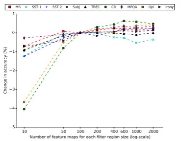
10 50 100 200 400 600 1000 2000 Number of feature maps for each filter region size (log-scale) 5
4 3 2 1 0 1
Change in accuracy (%)
MR SST-1 SST-2 Subj TREC CR MPQA Opi Irony
Figure 3: Effect of the number of feature maps.
the combination of several region sizes nearby this single best size, including combining both differ-ent region sizes and copies of the optimal sizes. 4.4 Effect of number of feature maps for
each filter region size
We again hold other configurations constant, and thus have three filter region sizes: 3, 4 and 5. We change only the number of feature maps for each of these relative to the baseline of 100; we con-sider values∈ {10, 50, 100, 200, 400, 600, 1000, 2000}. We report results in Fig.3.
The ‘best’ number of feature maps for each fil-ter region size depends on the dataset. However, it would seem that increasing the number of maps beyond 600 yields at best very marginal returns, and often hurts performance (likely due to overfit-ting). Another salient practical point is that it takes a longer time to train the model when the number of feature maps is increased.
In practice, the evidence here suggests perhaps searching over a range of 100 to 600. Note that this range is only provided as a possible standard trick when one is faced with a new similar sen-tence classification problem; it is of course possi-ble that in some cases more than 600 feature maps will be beneficial, but the evidence here suggests expending the effort to explore this is probably not worth it. In practice, one should consider whether the best observed value falls near the border of the range searched over; if so, it is probably worth ex-ploring beyond that border, as suggested in (
Ben-gio,2012).
4.5 Effect of activation function
Sigmoid function (Maas et al., 2013), SoftPlus function (Dugas et al.,2001), Cube function (Chen
and Manning,2014), and tanh cube function (Pei
et al., 2015). We use ‘Iden’ to denote the
iden-tity function, which means not using any activa-tion funcactiva-tion.
We show the numerical results of tanh, Softplus, Iden and ReLU in table6. For 8 out of 9 datasets, the best activation function is one of Iden, ReLU and tanh. The SoftPlus function outperform these on only one dataset (MPQA). Sigmoid, Cube, and tanh cube all consistently performed worse than alternative activation functions. The performance of the tanh function may be due to its zero cen-tering property (compared to Sigmoid). ReLU has the merits of a non-saturating form compared to Sigmoid, and it has been observed to accelerate the convergence of SGD (Krizhevsky et al.,2012). One interesting result is that not applying any acti-vation function (Iden) sometimes helps. This indi-cates that on some datasets, a linear transformation is enough to capture the correlation between the word embedding and the output label. However, if there are multiple hidden layers, Iden may be less suitable than non-linear activation functions. Prac-tically, with respect to the choice of the activation function in one-layer CNNs, our results suggest experimenting with ReLU and tanh, and perhaps also Iden.
4.6 Effect of pooling strategy
We next investigated the effect of the pooling strat-egy and the pooling region size. We fixed the filter region sizes and the number of feature maps as in the baseline configuration, thus changing only the pooling strategy or pooling region size.
In the baseline configuration, we performed 1-max pooling globally over feature maps, inducing a feature vector of length 1 for each filter. How-ever, pooling may also be performed over small equal sized local regions rather than over the en-tire feature map (Boureau et al.,2011). Each small local region on the feature map will generate a sin-gle number from pooling, and these numbers can be concatenated to form a feature vector for one feature map. The following step is the same as 1-max pooling: we concatenate all the feature vec-tors together to form a single feature vector for the classification layer. We experimented with local region sizes of 3, 10, 20, and 30, and found that 1-max pooling outperformed all local max pooling
configurations. This result held across all datasets. We also considered a k-max pooling strategy similar to (Kalchbrenner et al.,2014), in which the maximum k values are extracted from the entire feature map, and the relative order of these values is preserved. We explored thek∈ {5,10,15,20}, and again found 1-max pooling fared best, consis-tently outperformingk-max pooling.
Next, we considered taking an average, rather than the max, over regions (Boureau et al.,2010a). We experimented with local average pooling re-gion sizes {3, 10, 20, 30}. We found that aver-age pooling uniformly performed (much) worse than max pooling, at least on the CR and TREC datasets.
Our analysis of pooling strategies shows that 1-max pooling consistently performs better than al-ternative strategies for the task of sentence clas-sification. This may be because the location of predictive contexts does not matter, and certain
n-grams in the sentence can be more predictive on their own than the entire sentence considered jointly.
4.7 Effect of regularization
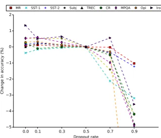
Two common regularization strategies for CNNs are dropout and l2 norm constraints; we explore the effect of these here. ‘Dropout’ is applied to the input to the penultimate layer. We experimented with varying the dropout rate from 0.0 to 0.9, fix-ing thel2norm constraint to 3, as per the baseline configuration. The results for non-static CNN are shown in in Fig.4, with 0.5 designated as the base-line. We also report the accuracy achieved when we remove both dropout and the l2 norm con-straint (i.e., when no regularization is performed), denoted by ‘None’.
Separately, we considered the effect of the
l2 norm imposed on the weight vectors that parametrize the softmax function. Recall that the
l2 norm of a weight vector is linearly scaled to a constraint c when it exceeds this threshold, so a smallerc implies stronger regularization. (Like dropout, this strategy is applied only to the penulti-mate layer.) We show the relative effect of varying
con non-static CNN in Figure 5, where we have fixed the dropout rate to 0.5; 3 is the baseline here (again, arbitrarily).
Dataset tanh Softplus Iden ReLU
MR 81.28 (81.07, 81.52) 80.58 (80.17, 81.12) 81.30 (81.09, 81.52) 81.16 (80.81, 83.38) SST-1 47.02 (46.31, 47.73) 46.95 (46.43, 47.45) 46.73 (46.24,47.18) 47.13 (46.39, 47.56)
SST-2 85.43 (85.10, 85.85) 84.61 (84.19, 84.94) 85.26 (85.11, 85.45) 85.31 (85.93, 85.66) Subj 93.15 (92.93, 93.34) 92.43 (92.21, 92.61) 93.11 (92.92, 93.22) 93.13 (92.93, 93.23) TREC 91.18 (90.91, 91.47) 91.05 (90.82, 91.29) 91.11 (90.82, 91.34) 91.54 (91.17, 91.84)
CR 84.28 (83.90, 85.11) 83.67 (83.16, 84.26) 84.55 (84.21, 84.69) 83.83 (83.18, 84.21) MPQA 89.48 (89.16, 89.84) 89.62 (89.45, 89.77) 89.57 (89.31, 89.88) 89.35 (88.88, 89.58) Opi 65.69 (65.16,66.40) 64.77 (64.25,65.28) 65.32 (64.78,66.09) 65.02 (64.53,65.45) Irony 67.62 (67.18,68.27) 66.20 (65.38,67.20) 66.77 (65.90,67.47) 66.46 (65.99,67.17)
Table 6: Performance of different activation functions
None 0.0 0.1 0.3 0.5 0.7 0.9 Dropout rate
4 3 2 1 0 1
Change in accuracy (%)
MR SST-1 SST-2 Subj TREC CR MPQA Opi Irony
Figure 4: Effect of dropout rate. The accuracy when the dropout rate is 0.9 on the Opi dataset is about 10% worse than baseline, and thus is not visible on the figure at this point.
imposing anl2norm constraint generally does not improve performance much (except on Opi), and even adversely effects performance on at least one dataset (CR).
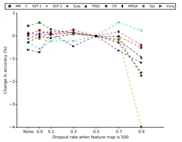
We then also explored dropout rate effect when increasing the number of feature maps. We in-crease the number of feature maps for each filter size from 100 to 500, and set max l2 norm con-straint as 3. The effect of dropout rate is shown in Fig. 6. We see that the effect of dropout rate is almost the same as when the number of feature maps is 100, and it does not help much. But we observe that for the dataset SST-1, dropout rate ac-tually helps when it is 0.7. Referring to Fig.3, we can see that when the number of feature maps is larger than 100, it hurts the performance possibly due to overfitting, so it is reasonable that in this case dropout would mitigate this effect.
We also experimented with applying dropout only to the convolution layer, but still setting the max norm constraint on the classification layer to 3, keeping all other settings exactly the same. This means we randomly set elements of the sentence matrix to 0 during training with probabilityp, and
1 2 3 4 5 10 15 20 25 30None l2 norm constraint on weight vectors 1.0
0.5 0.0 0.5 1.0
Change in accuracy (%)
MR SST-1 SST-2 Subj TREC CR MPQA Opi Irony
Figure 5: Effect of the l2 norm constraint on weight vectors.
None 0.0 0.1 0.3 0.5 0.7 0.9 Dropout rate when feature map is 500 4
3 2 1 0 1
Change in accuracy (%)
MR SST-1 SST-2 Subj TREC CR MPQA Opi Irony
Figure 6: Effect of dropout rate when using 500 feature maps.
em-0.0 0.1 0.3 0.5 0.7 0.9 Dropout rate
5 4 3 2 1 0 1 2
Change in accuracy (%)
MR SST-1 SST-2 Subj TREC CR MPQA Opi Irony
Figure 7: Effect of dropout rate on the convolution layer (The accuracy when the dropout rate is 0.9 on the Opi dataset is not visible on the figure at this point, as in Fig.4)
beddings helps to prevent overfitting (compared to bag of words based encodings). However, we are not advocating completely foregoing regular-ization. Practically, we suggest setting the dropout rate to a small value (0.0-0.5) and using a rela-tively large max norm constraint, while increasing the number of feature maps to see whether more features might help. When further increasing the number of feature maps seems to degrade perfor-mance, it is probably worth increasing the dropout rate.
5 Conclusions
We have conducted an extensive experimental analysis of CNNs for sentence classification. We conclude here by summarizing our main findings and deriving from these practical guidance for re-searchers and practitioners looking to use and de-ploy CNNs in real-world sentence classification scenarios.
From our experimental analysis we draw sev-eral conclusions that we hope will guide future work and be useful for researchers new to using CNNs for sentence classification.
• We find that, even when tuning them to the task at hand, the choice of input word vector representation (e.g., between word2vec and GloVe) has an impact on performance, how-ever different representations perform better for different tasks. At least for sentence classification, both seem to perform better than using one-hot vectors directly. Con-sider starting with the basic configuration described in Table 1 and using non-static word2vec or GloVe.
• The filter region size can have a large ef-fect on performance, and should be tuned. Line-search over the single filter region size to find the ‘best’ single region size. A rea-sonable range might be 1∼10. However, for datasets with very long sentences like CR, it may be worth exploring larger filter region sizes. Once this ‘best’ region size is iden-tified, it may be worth exploring combining multiple filters using regions sizes near this single best size, given that empirically multi-ple ‘good’ region sizes always outperformed using only the single best region size.
• 1-max pooling uniformly outperforms other pooling strategies.
• Consider different activation functions if pos-sible: ReLU and tanh are the best overall can-didates.
• Alter the number of feature maps for each fil-ter region size from 100 to 600, and when this is being explored, use a small dropout rate (0.0-0.5) and a large max norm constraint. Pay attention whether the best value found is near the border of the range (Bengio,2012). If the best value is near 600, it may be worth trying larger values.
• When assessing the performance of a model (or a particular configuration thereof), it is imperative to consider variance. Therefore, replications of the cross-fold validation pro-cedure should be performed and variances and ranges should be considered.
Of course, the above suggestions are applicable only to datasets comprising sentences with simi-lar properties to the those considered in this work. And there may be examples that run counter to our findings here. Nonetheless, we believe these sug-gestions are likely to provide a reasonable starting point for researchers or practitioners looking to ap-ply a simple one-layer CNN to real world sentence classification tasks.
We recognize that manual and grid search over hyperparameters is sub-optimal, and note that our suggestions here may also inform hyperparameter ranges to explore in random search or Bayesian optimization frameworks.
References
Yoshua Bengio. 2012. Practical recommendations for gradient-based training of deep architectures. In
Neural Networks: Tricks of the Trade, pages 437– 478. Springer.
Yoshua Bengio, R´ejean Ducharme, Pascal Vincent, and Christian Janvin. 2003. A neural probabilistic
lan-guage model. The Journal of Machine Learning
Re-search, 3:1137–1155.
James Bergstra, Daniel Yamins, and David Daniel Cox. 2013. Making a science of model search: Hyperpa-rameter optimization in hundreds of dimensions for vision architectures.
Y-Lan Boureau, Francis Bach, Yann LeCun, and Jean
Ponce. 2010a. Learning mid-level features for
recognition. InComputer Vision and Pattern
Recog-nition (CVPR), 2010 IEEE Conference on, pages 2559–2566. IEEE.
Y-Lan Boureau, Jean Ponce, and Yann LeCun. 2010b. A theoretical analysis of feature pooling in visual
recognition. In Proceedings of the 27th
Interna-tional Conference on Machine Learning (ICML-10), pages 111–118.
Y-Lan Boureau, Nicolas Le Roux, Francis Bach, Jean Ponce, and Yann LeCun. 2011. Ask the locals: multi-way local pooling for image recognition. In
Computer Vision (ICCV), 2011 IEEE International Conference on, pages 2651–2658. IEEE.
Thomas M Breuel. 2015. The effects of
hyperparam-eters on sgd training of neural networks. arXiv
preprint arXiv:1508.02788.
Danqi Chen and Christopher D Manning. 2014. A fast and accurate dependency parser using neural
net-works. InProceedings of the 2014 Conference on
Empirical Methods in Natural Language Processing (EMNLP), volume 1, pages 740–750.
Adam Coates, Andrew Y Ng, and Honglak Lee. 2011. An analysis of single-layer networks in unsuper-vised feature learning. In International conference on artificial intelligence and statistics, pages 215– 223.
Ronan Collobert and Jason Weston. 2008. A unified architecture for natural language processing: Deep
neural networks with multitask learning. In
Pro-ceedings of the 25th international conference on Machine learning, pages 160–167. ACM.
Ronan Collobert, Jason Weston, L´eon Bottou, Michael Karlen, Koray Kavukcuoglu, and Pavel Kuksa. 2011. Natural language processing (almost) from
scratch. The Journal of Machine Learning
Re-search, 12:2493–2537.
Charles Dugas, Yoshua Bengio, Franc¸ois B´elisle, Claude Nadeau, and Ren´e Garcia. 2001. Incorpo-rating second-order functional knowledge for
bet-ter option pricing. Advances in Neural Information
Processing Systems, pages 472–478.
Kavita Ganesan, ChengXiang Zhai, and Jiawei Han. 2010. Opinosis: a graph-based approach to abstrac-tive summarization of highly redundant opinions. In
Proceedings of the 23rd International Conference on Computational Linguistics, pages 340–348. Associ-ation for ComputAssoci-ational Linguistics.
Yoav Goldberg. 2015. A primer on neural network
models for natural language processing. arXiv
preprint arXiv:1510.00726.
Geoffrey E Hinton, Nitish Srivastava, Alex Krizhevsky, Ilya Sutskever, and Ruslan R Salakhutdinov. 2012. Improving neural networks by preventing
co-adaptation of feature detectors. arXiv preprint
arXiv:1207.0580.
Minqing Hu and Bing Liu. 2004. Mining and summa-rizing customer reviews. InProceedings of the tenth ACM SIGKDD international conference on Knowl-edge discovery and data mining, pages 168–177. ACM.
Mohit Iyyer, Varun Manjunatha, Jordan Boyd-Graber, and Hal Daum´e III. 2015. Deep unordered compo-sition rivals syntactic methods for text classification. Thorsten Joachims. 1998.Text categorization with sup-port vector machines: Learning with many relevant features. Springer.
Rie Johnson and Tong Zhang. 2014. Effective
use of word order for text categorization with
convolutional neural networks. arXiv preprint
arXiv:1412.1058.
Rie Johnson and Tong Zhang. 2015. Semi-supervised convolutional neural networks for text
categoriza-tion via region embedding. InAdvances in neural
information processing systems, pages 919–927. Nal Kalchbrenner, Edward Grefenstette, and Phil
Blun-som. 2014. A convolutional neural network for
modelling sentences. In Proceedings of the 52nd Annual Meeting of the Association for Computa-tional Linguistics (Volume 1: Long Papers), pages 655–665, Baltimore, Maryland. Association for Computational Linguistics.
Yoon Kim. 2014. Convolutional neural
net-works for sentence classification. arXiv preprint
arXiv:1408.5882.
Alex Krizhevsky, Ilya Sutskever, and Geoffrey E Hin-ton. 2012. Imagenet classification with deep
con-volutional neural networks. In Advances in neural
information processing systems, pages 1097–1105. Yann LeCun, Yoshua Bengio, and Geoffrey Hinton.
2015. Deep learning. Nature, 521(7553):436–444.
Xin Li and Dan Roth. 2002. Learning question
clas-sifiers. In Proceedings of the 19th international
Andrew L Maas, Awni Y Hannun, and Andrew Y Ng. 2013. Rectifier nonlinearities improve neural
net-work acoustic models. InProc. ICML, volume 30.
Tomas Mikolov, Ilya Sutskever, Kai Chen, Greg S Cor-rado, and Jeff Dean. 2013. Distributed representa-tions of words and phrases and their
compositional-ity. InAdvances in neural information processing
systems, pages 3111–3119.
Bo Pang and Lillian Lee. 2005. Seeing stars: Exploit-ing class relationships for sentiment categorization with respect to rating scales. InProceedings of the ACL.
Wenzhe Pei, Tao Ge, and Baobao Chang. 2015. An effective neural network model for graph-based de-pendency parsing. InProc. of ACL.
Jeffrey Pennington, Richard Socher, and Christo-pher D Manning. 2014. Glove: Global vectors for
word representation. Proceedings of the Empiricial
Methods in Natural Language Processing (EMNLP 2014), 12:1532–1543.
David E Rumelhart, Geoffrey E Hinton, and Ronald J Williams. 1988. Learning representations by back-propagating errors.Cognitive modeling, 5:3.
Richard Socher, Alex Perelygin, Jean Y Wu, Jason Chuang, Christopher D Manning, Andrew Y Ng, and Christopher Potts. 2013. Recursive deep models for semantic compositionality over a sentiment tree-bank. InProceedings of the conference on empirical methods in natural language processing (EMNLP), volume 1631, page 1642. Citeseer.
Nitish Srivastava, Geoffrey Hinton, Alex Krizhevsky, Ilya Sutskever, and Ruslan Salakhutdinov. 2014. Dropout: A simple way to prevent neural networks
from overfitting. The Journal of Machine Learning
Research, 15(1):1929–1958.
Byron C Wallace, Laura Kertz Do Kook Choe, and Eu-gene Charniak. 2014. Humans require context to infer ironic intent (so computers probably do, too). In Proceedings of the Annual Meeting of the Asso-ciation for Computational Linguistics (ACL), pages 512–516.
Byron C Wallace, Kevin Small, Carla E Brodley, and Thomas A Trikalinos. 2011. Class imbalance,
re-dux. InData Mining (ICDM), 2011 IEEE 11th
In-ternational Conference on, pages 754–763. IEEE.
Peng Wang, Jiaming Xu, Bo Xu, Chenglin Liu, Heng Zhang, Fangyuan Wang, and Hongwei Hao. 2015.
Semantic clustering and convolutional neural net-work for short text categorization. InProceedings of the 53rd Annual Meeting of the Association for Computational Linguistics and the 7th International Joint Conference on Natural Language Processing (Volume 2: Short Papers), pages 352–357, Beijing, China. Association for Computational Linguistics.
Janyce Wiebe, Theresa Wilson, and Claire Cardie. 2005. Annotating expressions of opinions and
emo-tions in language. Language resources and
evalua-tion, 39(2-3):165–210.
Dani Yogatama and Noah A Smith. 2015. Bayesian optimization of text representations. arXiv preprint arXiv:1503.00693.
Ye Zhang, Matthew Lease, and Byron C Wallace. 2017. Exploiting domain knowledge via grouped weight sharing with application to text categoriza-tion. arXiv preprint arXiv:1702.02535.
Ye Zhang, Stephen Roller, and Byron Wallace. 2016. Mgnc-cnn: A simple approach to exploiting mul-tiple word embeddings for sentence classification.