A Study on Evaluation of Seismic Response considering Basemat Uplift
for Soil-building System using 3D FEM
Takeshi Kawasato 1), Tetsuya Okutani 1), Osamu Kurimoto 2) and Masahito Akimoto 3)
1) Project Development Department, The Japan Atomic Power Company, Japan 2) Technical Research Institute, Obayashi Corporation, Japan
3) Nuclear Facilities Division, Obayashi Corporation, Japan
ABSTRACT
Basemat uplift of a structure is an important problem in seismic design for nuclear facilities. It has been evaluated from the dynamic response of a structure using a Sway-Rocking (SR) model. However, it is pointed out that the accuracy of this model decreases as the uplift becomes large. This paper describes the seismic response of a soil-structure system using a three-dimensional finite element method, which will be useful to evaluate nonlinear phenomena.
1 INTRODUCTION
The evaluation of dynamic responses of nuclear power plants (NPP) considering of the soil-structure interaction (SSI) is strictly required for seismic design in Japan. A sway-rocking (SR) model is often used, and the soil springs are estimated from the vibration admittance theory (VA), which is based on the three dimensional wave propagation theory for the uniform half-space soil medium. The basemat uplift is also considered in a rotational soil spring with the geometry nonlinear characteristics. While the dynamic response analysis using SR model is a simple procedure, it is difficult to express basemat uplift nonlinearity for the complex site conditions such as embedment effects.
A three dimensional finite element method (3D FEM) is one of the most effective methods in case of complicated geometry. In recent years the performance of computers has been improved remarkably, it would be possible to use a large scale 3DFE model in the practical seismic design. However, FE model is faced with a problem of 'finite boundaries', and viscous boundary is used to make a model of infinite half space soil medium in time domain dynamic analysis. It should be necessary to investigate the validity of soil model. In addition, joint elements are adopted in FE analysis to express basemat uplift, and the stability and the accuracy of analytical solutions should be verified. This paper describes a procedure to make a proper numerical modeling technique when using 3D FEM for the infinite half space soil medium and analysis results of dynamic response of NPP considering basemat uplift by using joint elements in 3D FE soil model.
2 IMPEDANCE AND FOUNDATION INPUT MOTION
In this chapter, the proper modeling of an infinite half space soil medium in 3D FEM is discussed. The impedance and the foundation input motion which are basic properties of SSI, can be evaluated by a various approach. First, the exact solutions of them are evaluated by VA, and next, the properness of 3D soil model is confirmed by comparing the solutions by 3D FEM with those by VA.
2.1 EVALUATION PROCEDURE
1D wave
propagation theory Free field Comparison of foundation input motion and original wave motion
Near field soil media h=1%
5.00 0.02 0.10 1.00 3000
0 2000 1000
Original wave motion
ORIGINAL
5.00 0.02 0.10 1.00 3000
0 2000 1000
Foundation input motion
Far field soil media
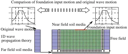
Fig. 1 Evaluation Procedure of Base Input Motion The verification procedure for evaluating the
foundation input motion is illustrated in Fig 1. First, the earthquake ground motion at the surface of far field soil is defined (this wave is called ‘original wave motion’ afterward). Second, the earthquake wave at the lower edge level of 3D FE soil model is defined by 1D wave propagation theory, and is input into 3D FE soil model. The response at the surface level is evaluated as the foundation input motion of the structure when the
earthquake is input with right angle and the basemat embedment is not considered. Therefore, the proper modeling can be confirmed by comparing the soil surface response with the original wave motion.
The next verification procedure for evaluating the impedance function is shown in Fig 2. Several sine-wave force time histories, whose frequencies are different, are prepared and a series of dynamic analyses are performed by applying the sine-wave force time histories in order to obtain the responses at the soil surface. The impedance function is defined from the relationship between the
response displacement and the applied force. Consequently the impedance function is verified by comparing with an exact solution obtained by using VA.
Elastic spring with the same stiffness of the initial stiffness of the Joint element
Sinusoidal exciting force
3D FE Soil model
Foundation area
3D FE Soil model
a. Impedance Function b. Initial Stiffness of Joint Element Fig. 2 Evaluation Procedure of Impedance Function and
Furthermore, the proper determination of initial stiffness of a joint element is verified on basemat uplift in 3D FE analysis. Although the initial stiffness of joint element is desirable to be infinite theoretically, the numerical analysis with joint element tends to be unstable when the larger value is adopted as an initial stiffness of joint element. Therefore, the initial stiffness of joint element should be chosen the suitable value where the analysis will not become unstable. However, the criteria of choosing the suitable value have not been clear yet. A series of dynamic analyses which are similar to the evaluation of impedance function mentioned above are performed by applying the sine-wave force time histories to an end of the joint elements, which is not connected with soil medium directly, as shown in the right figure of Fig. 2. These analyses reveal the influence of the joint elements on impedance function, and the criteria for the initial stiffness of a joint element comparing with the results which were applied sine-wave force time histories to the soil medium directly.
2.2 ANALYTICAL MODEL
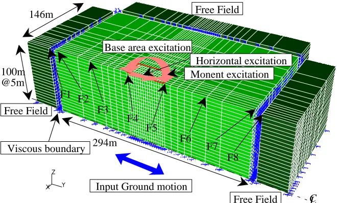
The 1/2 symmetry condition is adopted to construct an analytical model about a soil medium of 3D FEM as shown in Fig. 3. Brick elements are used to model a soil medium and the near field soil and the far field soil are connected by using dashpots as viscous boundaries. However, the analytical soil medium model without the far field parts is used when the impedance evaluation is performed because it is required to consider only wave dissipation from the interior region of soil medium. In other words the outside of dashpots is treated as fixed boundaries in the impedance analysis. The P-wave and S-wave velocity of the soil medium in this study are Vp=3700m/s and Vs=1800m/s, respectively, and the material damping of soil medium is not considered.
Free Field
Base area excitation
Input Ground motion
294m
100m
@5m
146m
F1 F2
F3
F4
F8
F7
F6
F5
C
L
Monent excitation
Viscous boundary
Free Field
Free Field
Horizontal excitation
Fig. 3 3D-FE Model of Soil System
2.3 FOUNDATION INPUT MOTION
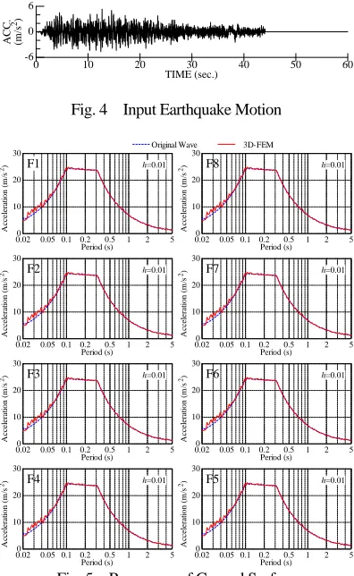
The acceleration time histories, which are used as the original wave motion, are shown in Fig.4. The acceleration responses at the surface of the soil medium are evaluated with this input motion following the procedure illustrated in Fig.1. The points, at which the acceleration responses are evaluated, are selected on the line which goes through the center of the basemat. And these acceleration responses of each point are compared with the original wave motion in the acceleration response spectra of damping factor h=1%. The responses of representative evaluation point from F1 through F8 are shown in Fig. 5. The acceleration response spectrum of the original wave motion is expected to be coincident with that of each point if a soil medium is homogeneous and the basemat is not embedded. From Fig. 5, it can be recognized that the responses, which are evaluated at the points from F1 through F8, are almost equal to the original wave motion. Therefore, it can be confirmed that the foundation input motion is expressed accurately by using 3D FE soil model, and it can be found that the analytical model of a soil medium constructed in this study is proper.
0 10 20 30 40 50 60
-6 0 6
ACC. (m/s
2)
TIME (sec.)
Fig. 4 Input Earthquake Motion
0.020 0.05 0.1 0.2 0.5 1 2 5 10
20 30
A
ccel
er
at
io
n (
m
/s
2)
Period (s)
Original Wave 3D-FEM h=0.01
F1
0.020 0.05 0.1 0.2 0.5 1 2 5 10
20 30
A
ccel
er
at
ion
(
m
/s
2)
Period (s) h=0.01 F2
0.020 0.05 0.1 0.2 0.5 1 2 5 10
20 30
A
ccel
er
at
io
n
(
m
/s
2)
Period (s) h=0.01 F3
0.020 0.05 0.1 0.2 0.5 1 2 5 10
20 30
A
cc
el
era
ti
o
n
(m
/s
2)
Period (s) h=0.01 F4
0.020 0.05 0.1 0.2 0.5 1 2 5 10
20 30
A
cc
el
era
ti
o
n
(m
/s
2)
Period (s) h=0.01 F5
0.020 0.05 0.1 0.2 0.5 1 2 5 10
20 30
A
ccel
er
at
io
n
(
m
/s
2)
Period (s) h=0.01 F6
0.020 0.05 0.1 0.2 0.5 1 2 5 10
20 30
A
ccel
er
at
ion
(
m
/s
2)
Period (s) h=0.01 F7
0.020 0.05 0.1 0.2 0.5 1 2 5 10
20 30
A
ccel
er
at
io
n (
m
/s
2)
Period (s) h=0.01 F8
Fig. 5 Responses of Ground Surface 2.4 IMPEDANCE FUNCTION
To evaluate the horizontal impedance function using 3D FE soil model, the uniformly distributed horizontal sine-wave force time histories are applied to the area, where the basemat exists and dynamic time-history analyses, are performed. The maximum horizontal displacement responses evaluated at the grids in the basemat area are averaged. A complex horizontal impedance function is expressed in KH=Qexp(iφ)/U, when Q is the sum of the amplitude of the applied sine-wave force time histories and U is the average of the maximum displacement responses and φ is the phase lag between the applied force time histories and the average displacement response time histories. The relationship of the three parameters Q, U and φ mentioned above is shown in Fig. 6.
Similarly, to evaluate rotational impedance function, the skew symmetrically distributed triangular vertical sine-wave force time histories are applied to the area where the basemat exists, and dynamic time-history analyses are performed. Here, to evaluate an averaged basemat rotational angle, the maximum vertical displacement responses evaluated at the grids in this area are averaged by considering the amplitude of the applied force time histories as the weight.
The couple of impedance functions for each frequency are evaluated by repeating the procedure mentioned above, using a series of applied force time histories with different frequencies.
The complex impedance functions evaluated by 3D FEM, which are being compared with those evaluated by VA, are shown in Fig. 7. To evaluate the impedance functions by VA, the analyses under two different assumptions are performed. One assumption is that the soil reaction under the basemat is uniformly distributed, and the other is that the amplitude distribution of the displacement responses under the basemat is uniform. The latter assumption corresponds to the case of the rigid basemat. It
Si
n
u
so
id
a
l
Ex
ci
tat
io
n Sinusoidal Excitation Q
Phase Lag ϕ
Re
sp
ons
e
D
is
p
la
cemen
t
TIME TIME
Response Displacement U
Fig. 6 Evaluation Procedure of Impedance Function
can be recognized that the horizontal impedance function evaluated by FEM is approximately equal to that evaluated by VA and that both of them have the same tendency concerning to the evaluated values, which are consist of the real and the imaginary part, and the dependency to the frequencies. Similarly, about the rotational impedance functions, it would be possible to conclude that the results evaluated by 3D FEM almost correspond to those of VA, but when looking at the comparison in detail, the former seem to be dependent to frequencies more strongly than the latter.
2.5 INITIAL STIFFNESS OF JOINT ELEMENT
To determine proper value of the initial stiffness of joint element, a series of impedance analyses are performed by changing the initial stiffness of joint elements as a parameter. When the parametric analyses mentioned are performed, the impedance function at 0Hz evaluated by VA is treated as a basis, which is considered the static soil stiffness.
The results are shown in Fig. 8. While 5 times of the static soil stiffness is adopted as the initial stiffness of the joint elements, the evaluated values are much smaller than those which are evaluated by applying the sine-wave force time histories to the soil medium directly. While 50 times or 100 times of the static soil stiffness is adopted as the initial stiffness of the joint elements, the former are almost the same level of the latter. Therefore, in order to preserve the soil-foundation interaction characteristics for the example of this study, it can be recognized that the value which is almost 50 times of the static soil stiffness must be set as the initial stiffness of joint elements.
3 BASEMAT UPLIFT CHARACTERISTICS
Based on the Mindlin's solutions derived from the three dimensional elasticity theory or the Green function method, Tanaka et al constructed the evaluation method for the uplift characteristics of the structures to which the seismic excitations are applied, and they arranged this method to be applied to SR model which is often used in the SSI analyses. In Japan, this procedure which was proposed by Tanaka et al (1995) is used as the existing structural design method for NPP facilities.
0 5.0 10.0 15.0 20.0 0
1.0 2.0 3.0 4.0
VA : given displacements are uniformly distrbuted VA : given soil reactions are uniformly distrbuted 3D FEM
[×109]
KH
(k
N
/m
)
FREQUENCY (Hz) Horizontal Components
0 5.0 10.0 15.0 20.0 0
0.5 1.0 1.5 2.0[×10
12]
KR
(k
N
·m
)
FREQUENCY (Hz) Rotational Components
Fig. 7 Comparison of Impedance Functions obtained from 3D-FEM and VA
0 5.0 10.0 15.0 20.0 0
1.0 2.0 3.0
4.0[×109] 2.0
In this chapter, the relation between the basemat-overturning-moment and the basemat rotational angle and the contact ratio (M-θand M-η) are evaluated by performing the static and dynamic analyses based on 3D FEM, and the relation between the solutions evaluated by 3D FEM and the existing structural design method are studied. The static and dynamic M-θ and M-η relations are quantitatively characterized.
3.1 EVALUATION PROCEDURE
Now, the massless rigid base, which consists of the brick elements, is added to the soil model used in Chapter 2 (in Fig. 3 ), and this rigid base is connected to the soil medium by introducing the joint elements between them. Then, to evaluate the rotation angle response of the base, the overturning moment is applied to it, and a static or dynamic time-history analysis is performed. In the case of the static analysis, the overturning moment is applied to the base gradually for each loading step, and in the case of the dynamic analysis, the sine wave moment time histories are used. TTo recognize the basemat uplift nonlinear characteristics clearly, the overturning moment mentioned above is appleid to the base until the contact ratio reaches about 40%.
H
o
ri
zont
al
C
o
m
pon
ent
KH
(k
N
/m
)
Frequency (Hz) Kr(Direct Excitation) Ki(Direct Excitation) Kr(5 times to initial stiffness) Ki(5 times to initial stiffness) Kr(10 times to initial stiffness) Kr(10 times to initial stiffness) Kr(50 times to initial stiffness) Kr(50 times to initial stiffness) Kr(100 times to initial stiffness) Kr(100 times to initial stiffness)
0 5.0 10.0 15.0 20.0 0
0.5 1.0 1.5
[×1012]
R
o
ta
tio
n
al C
o
m
p
o
n
en
t
KR
(k
N
·m
)
Frequency (Hz)
Fig. 8 Influence to Impedance Functions due to Initial Stiffness of Joint Elements
294m 100m
@5m 146m
CL
Base area excitation
Basemat
Fig. 9 3D-FE Model of Soil-Foundation System
Massless rigid foundation
Joint element Static analysis Dynamic analysis
Moment excitaton STEP
M
TIME M Sinusoidal exciting force
Gradually increasing force
Soil media model
Fig. 10 Analysis Procedure of M-θ and M-η Relationships
3.2 STATIC BASEMAT UPLIFT CHARACTERISTICS
In Fig.11, the static M-θ and M-η relations evaluated by the procedure mentioned above are shown, comparing them with those calculated from the proposed equations used in the existing structural design method for NPP facilities in Japan.
Tanaka et al (1995) proposed the following equations to express the base uplift nonlinear characteristics which they intended to give to the rotational soil spring in SR model.
Angle Rotational Bound
Uplift
width Base L weight Base W
M M WL M
:
: , :
, 2
2 2 ,
0
2 2 0 2 2 0
0 0
θ
θ θ η θ θ α α α
α
α− −
⎟ ⎠ ⎞ ⎜ ⎝ ⎛ = ⎟ ⎠ ⎞ ⎜ ⎝ ⎛ − − = =
(1)
In this equation, α is a parameter which shows the reaction distribution under the base. In the case of α=6, this equations become the following familiar form which can be easily derived from the assumption that both the reaction and the vertical displacement distributions of the base are triangular.
θ θ η θ
θ0 0
0
0 , 3 2 ,
6 = − =
=
M M WL
M (2)
Moreover, in the case of the rigid base, α equals 4.7, which was decided in order that the calculation results by this equation accord with those evaluated from the analysis based on the Green
function method. In addition, the Eq. 2 are usually used in the structural design of NPP in Japan.
0 1.0 2.0 3.0
0 0.5 1.0 1.5 2.0
θ0=4.76×10⁻⁶(α=6.0)
θ0=6.08×10⁻⁶(α=4.7)
θ0=6.13×10⁻⁶(3D-FEM)
Rotaional Angle θ (rad.)
O
ve
rt
ur
n
in
g M
om
ent
M
(
k
N
·m
) M
0=7.72×10⁶kN·m(3D-FEM)
M0=7.65×10⁶kN·m(α=4.7)
M0=6.00×10⁶kN·m(α=6.0)
3D-FEM
Proposed by Tanaka et al. (α=4.7)
Proposed by Tanaka et al. (α=6.0)
that is equivalent to conventional method
[×10-5]
[×107]
0 0.5 1.0 1.5 2.0
0 0.2 0.4 0.6 0.8 1.0 1.2
Overturning Moment M (kN·m)
Co
n
ta
ct
Ra
ti
o
η
M0(α=6.0)
M0(α=4.7)
M0(3D-FEM)
[×107]
Fig. 11 Static M-θ and M-η Relationships
It can be recognized that the static M-θ and M-η relations evaluated by 3D FEM have the uplift characteristics almost corresponding to those in the case of α=4.7 of the existing structural design method. On the other hand, when comparing the results of 3D FEM with those in the case of α=6, it can be said that the uplift bound moment M0 of the former is larger than that of the latter and that the progress of the uplift of the former is slower than that of the latter.
3.3 DYNAMIC BASEMAT UPLIFT CHARACTERISTICS
The 3D dynamic analyses are performed by applying the sine wave moment time histories of the frequency 1Hz, 5Hz and 10Hz to the base. The time histories of the overturning moment, the rotational base angle and the contact ratio are shown in Fig. 12, and the dynamic M-θ and M-η relations are shown in Fig. 13.
0 5 10 15 -2.0 -1.0 0 1.0 2.0 O v er tu rn ing M o m ent M (k N ·m )
[×107]
0 5 10 15
-3.0 -2.0 -1.0 0 1.0 2.0 3.0 R o ta tio n al A n g le θ (ra d .)
[×10-5]
0 5 10 15
0 0.2 0.4 0.6 0.8 1.0 C ont ac t R at io η TIME (s)
0 1 2 3
-2.0 -1.0 0 1.0 2.0[×107]
0 1 2 3
-3.0 -2.0 -1.0 0 1.0 2.0 3.0[×10-5]
0 1 2 3
0 0.2 0.4 0.6 0.8 1.0 TIME (s)
0 0.5 1 1.5
-2.0 -1.0 0 1.0 2.0[×107]
0 0.5 1 1.5
-3.0 -2.0 -1.0 0 1.0 2.0 3.0[×10-5]
0 0.5 1 1.5
0 0.2 0.4 0.6 0.8 1.0 TIME (s)
(a) 1Hz (b) 5Hz (c) 10Hz Fig. 12 Time Histories of Overturning Moment, Rotational Angle and Contact Ratio
-3.0 -2.0 -1.0 0 1.0 2.0 3.0 -2.0 -1.5 -1.0 -0.5 0 0.5 1.0 1.5 2.0
Rotaional Angle θ (rad.)
O v er tu rn in g M o m en t M ( k N ·m )
[×107]
[×10-5] -2.0 -1.0 0 1.0 2.0
0 0.2 0.4 0.6 0.8 1.0
Overturning Moment M (kN·m)
Co n ta ct Ra ti o η
[×107]
(a) Exciting Frequency : 1Hz
-3.0 -2.0 -1.0 0 1.0 2.0 3.0 -2.0 -1.5 -1.0 -0.5 0 0.5 1.0 1.5 2.0
Rotaional Angle θ (rad.)
O v er tu rn in g M o m en t M ( k N ·m )
[×107]
[×10-5] -2.0 -1.0 0 1.0 2.0
0 0.2 0.4 0.6 0.8 1.0
Overturning Moment M (kN·m)
Co n ta ct Ra ti o η
[×107]
(b) Exciting Frequency : 5Hz
-3.0 -2.0 -1.0 0 1.0 2.0 3.0 -2.0 -1.5 -1.0 -0.5 0 0.5 1.0 1.5 2.0
Rotaional Angle θ (rad.)
O v er tu rn in g M o m en t M ( k N ·m )
[×107]
[×10-5] -2.0 -1.0 0 1.0 2.0
0 0.2 0.4 0.6 0.8 1.0
Overturning Moment M (kN·m)
Co n ta ct Ra ti o η
[×107]
(c) Exciting Frequency : 10Hz
Fig. 13 Dynamic M-θ and M-η Relationships First, from the responses in the case of 1Hz sine wave
moment time histories, the rotational angle time histories have almost sine waveform before the base uplift begins, but their waveform becomes warped and triangular as the base uplift proceeds. The progress and repetition of the base uplift event can be recognized from the contact ratio time histories. The dynamic M-θ and M-η relations of the case of 1Hz is considered to be almost the same of the static relations, judging from the situation that they have the hysteresis which is made by expanding the static relations in centrosymmetry for the origin. For the case of applying the 1Hz excitation, the soil medium with the shear velocity speed Vs=1800m/s may be too hard to expect the energy dissipation effect to it.
Next, from the responses in the case of 5Hz sine wave moment time histories, the rotational angle time histories waveform becomes triangular as the base uplift proceeds, as is in the case of 1Hz excitation. The Contact ratio time histories of the case of 5Hz excitation are similar to those of the case of 1Hz excitation in the time zone of the neighborhood where the maximum base uplift is generated, but they are not stable in the time zone where the base lands on the soil medium again. This tendency appears remarkable in the case of 10Hz excitation. In this case, the contact ratio is almost 80% (in other words, the base uplift ratio is almost 20%), in the time zone when the base is expected to contact the soil medium perfectly. The self-exciting oscillation caused by the base uplift event may be generated at the surface of the soil medium.
Finally, from the responses in the case of 10Hz sine wave moment time histories, it can be found that the energy dissipation effect of the soil medium from the dynamic M-θ relation is larger than that in the case of 1Hz excitation. The shape of this M-θ relation is oval until the base uplift begins. After the base uplift progress, it keeps a fixed quantity of hysteresis area though the peaks of hysteresis become sharp. The energy dissipation effect may be found from the dynamic M-η relation, but it must be paid attention to the fact that the energy dissipation effect judged from the dynamic M-η relation is bigger than the real energy dissipation. As mentioned above, there are some joint elements which show the takeoff situation because of the self-exciting oscillation at the surface of the soil medium in the time zone when the contact ratio is considered 100% .
4 DYNAMIC ANALYSES FOR SOIL-FOUNDATION-BUILDING SYSTEM USING 3D FE MODEL
In this chapter, the dynamic time histories analyses are performed for the soil-foundation-building System by 3D FE soil model and SR model, and these results are compared. The S-wave velocity of the soil medium in this study is Vs=1800m/s, and the base of building is assumed to be rigid. The input earthquake motion used here is shown in Fig. 4.
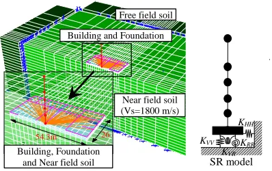
4.1 ANALYTICAL MODEL
3D FE soil model and SR model are shown in Fig. 14. The 5 stories building which consists of a top steel story and four reinforced concrete stories is considered here. This is composed as a stick model, and used in the both analyses. In SR model, the horizontal, rotational and vertical impedance functions evaluated by VA are attached at the base bottom of the building. Furthermore, in 3D FE soil model, several rigid beam elements are used to connect the building model mentioned above and the base which consist of rigid brick elements at the surface of a soil model. These rigid beam elements are expected to transmit the shear force and the bending moment generated in the building caused by the seismic excitation to the base. Joint elements are put between the building base and the surface of the soil medium in order to consider the base uplift. As the initial stiffness of joint
elements, a value of 100 times of the static soil spring is used. The other elements except joint elements are assumed to be linear materials.
Near field soil (Vs=1800 m/s) Free field soil Building and Foundation
54.3m 26.6
建屋・基礎・近傍地盤Bu
KHH
KVV KRR
4.2 ANALYSIS RESULTS
In Figs.15 through 17, the building responses evaluated by 3D FE soil model are compared with those evaluated by SR model.
The maximum responses about the horizontal and vertical acceleration, the shear force and the bending moment in the both analyses are shown in Fig.15. From the horizontal responses, the evaluated values by both analyses are almost same, but a slight difference may be found in the horizontal maximum acceleration of the top of building, and in the maximum shear force responses. This may come from the fact that the different type of damping is used in both analyses. In this study, the stiffness proportional damping is assumed in the 3D FE soil model, and the strain energy proportional damping is adopted in SR model. About the vertical responses, the evaluated values and their distributions by both analyses are approximately equal except the base response. A pulsing response may be observed at the base in 3D FE soil model,
which couldn't be found in SR model. The up-and-down responses generated by base uplift and their mechanism must be scrutinized in the future.
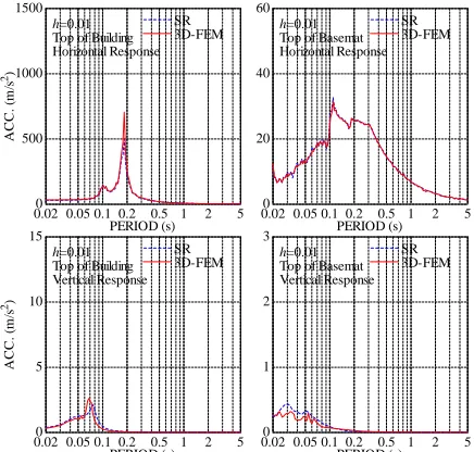
The horizontal and vertical acceleration response spectra at the top of building and the base top surface are shown in Fig.16. About the horizontal responses, some slight distinctions can be seen in the peak value around 0.2 second at the top of building, and the value evaluated by 3D FE soil model is larger than that evaluated by SR, but the spectral characteristics in the both
ilding, Foundation and Near field soil
KVR
SR model
Fig. 14 3D-FE Model of Soil-Foundation-Building System
0 10 20 30 40 50 0
5 10 15 20 25 30 35
E
levat
io
n (
m
)
Max. Horizontal Accelerration (m/s 2) SR 3D-FEM
0 0.5 1 1.5 2 0
5 10 15 20 25 30 35
Max. Vertical Accelerration (m/s 2) SR 3D-FEM
0 20 40 60 80 0
5 10 15 20 25 30 35
E
levat
io
n (
m
)
Max. Shear Force (×104 kN) SR 3D-FEM
0 50 100 150
0 5 10 15 20 25 30 35
Max. Bending Moment (×10 5 kN·m) SR 3D-FEM
Fig. 15 Comparizon of Maximum Responses
analyses is approximately equal, and the responses at the base top surface are particularly equivalent from the viewpoint of both the amplitude and the period. About the vertical responses, the evaluated acceleration response spectra by both SR model and 3D FE soil model are approximately equal all over the period. The time histories of the contact ratio evaluated by both analyses are shown in Fig.17. The time when the base uplift is generated in the both analyses is approximately equal. The minimum contact ratio in 3D FE soil model is smaller than that in SR model. This may show that the base uplift is harder to be generated in 3D FE soil model than in SR model.
0.02 0.05 0.1 0.20 0.5 1 2 5 500
1000 1500
ACC.
(
m
/s
2)
SR 3D-FEM h=0.01
Top of Building Horizontal Response
PERIOD (s) 0.02 0.05 0.1 0.2 0.5 1 2 5 0
20 40 60
SR 3D-FEM h=0.01
Top of Basemat Horizontal Response
PERIOD (s)
0.02 0.05 0.1 0.20 0.5 1 2 5 5
10 15
A
CC.
(
m
/s
2)
SR 3D-FEM h=0.01
Top of Building Vertical Response
PERIOD (s) 0.02 0.05 0.1 0.2 0.5 1 2 5 0
1 2 3
SR 3D-FEM h=0.01
Top of Basemat Vertical Response
PERIOD (s)
Fig. 16 Comparizon of Acceleration Response Spectra
0 10 20
0.5 0.6 0.7 0.8 0.9 1.0
C
o
n
ta
ct R
atio
η
3D-FEM SR
TIME (s)
Fig. 17 Comparizon of Time History of Contact Ratio
5 CONCLUDING REMARKS
This paper described precise analysis results using 3D FEM on seismic response of NPP considering basemat uplift. The evaluation procedure for the analysis model and parameters is proposed and verified through comparison with impedance functions, foundation input motions, nonlinear M-θ relationships and nonlinear seismic responses. Remarkable results obtained in this study are as follows.
1. The initial stiffness of joint elements should be set to more than 50 times of the static soil spring where the existence joint elements would not change the dynamic soil-structure interaction characteristics
2. The static M-θ relationship obtained from 3D FE soil model shows good coincidence with that obtained 3D elastic theory using Mindlin's solutions. The dynamic M-ηrelationship shows the peculiar nonlinear characteristics which caused by basemat uplift.
3. Both 3D FE soil model and SR model give almost equal maximum responses and the response spectra of the building with basemat uplift.
4. It is found that 3D FE soil model could be useful technique to evaluate basemat uplift. It would be applicable to full and partial embedded foundations where it is difficult to apply SR model.
REFERENCES
1) Japan Electric Association (JEA), Technical Guidelines for Aseismic Design of Nuclear Power Plants, JEAG 4601-1991 Supplement (in Japanese).
2) Tajimi,H., Interaction of Building and Ground, Earthquake Engineering, Shokokusha Publishing Co., 1968
3) Tnaka,H., Maeda,I., Moriyama,K., Watanabe,S., Study on horizontal-vertical interactive SR model for basemat uplift(Part1 & Part2) ,Trans. of SMiRT 13, Vol. K, 1995, pp43~54