Characterization of the Vertical Seismic Coefficient
for Pseudo-Static Slope Stability Analysis
Jongmin Kim1, Sangho Choi2
1 Assist. Professor, Dept. of Civil and Environmental Eng, Sejong Univ., Seoul, Korea, ([email protected]) 2 Researcher, Korean Infrastructure Safety and Technology Corporation, Goyang, Gyeonggi-do, Korea
ABSTRACT
Seismic load applied to slope seismic analysis can be divided into horizontal and vertical seismic load. Vertical seismic load is often ignored because it is relatively small in magnitude compared to horizontal seismic load. But considering that the Kobe earthquake (1995, M=7.2), the Chile earthquake (2010, M=8.8) and the Christchurch earthquake (2010, M=6.6) each had an epicenter that occurred in an inland area or a coastal area close to inland, and analysis of their seismic wave component shows that vertical ground acceleration is similar to or greater than horizontal ground acceleration, both horizontal and
vertical seismic load should be considered in slope seismic analysis based on seismic wave component. While horizontal seismic load can be calculated from the seismic coefficient offered in the design guideline, previous studies and design guidelines have only covered the magnitude and direction of vertical seismic load. For this reason, there are many difficulties in applying horizontal seismic load in slope seismic analysis. Thus, this study completes the limit analysis program using objective function which is seismic coefficient ratio expressed by a function of horizontal and vertical seismic load and analyses the relation between horizontal seismic coefficient and seismic coefficient ratio setting the horizontal seismic coefficient(kh), the inclination of slope(), the friction coefficient(), the safety
number(Nc) as a parameter. It was found that the influence of combined seismic force on slope stability
shows three different tendencies, and limit equilibrium analysis is performed to verify these tendencies.
INTRODUCTION
vertical inertia force, destabilizing the slope, is proposed as well. Either upward or downward direction is specified as a unfavorable to stability with regard to the conditions of slope and earthquake loading.
FORMULATION OF LIMIT ANALYSIS CONSIDERING COMBINED SEISMIC FORCE
DESCRIPTION OF LIMIT ANALYSIS
Limit analysis can be divided into upper-lower bound analysis, and is an analysis technique used to compute the upper-lower bound value of a stability problem. Lower bound analysis enables the computation of lower bound value for mechanically rigorous failure conditions by assuming statically admissible stress field satisfied with Mohr-Coulomb's yield criterion , equilibrium condition and stress boundary condition at every node that constitute given soil mass. Upper bound analysis enables the computation of upper bound value for mechanically rigorous failure conditions by assuming kinematically admissibility velocity fields satisfied with principle virtual work, compatibility condition, flow rule and velocity boundary condition on every node that constitute given soil mass. Therefore, limit analysis involves calculating mechanically rigorous lower bound solution and upper bound solution. Finite element, which is expressed by a linear shape function, is used to apply assumptions of limit analysis, and Steepest edge active set algorithm is applied in order to compute the optimum solution (Sloan, 1988, 1989; Sloan and Kleeman, 1995).
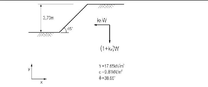
Statically admissible stress field in lower bound analysis considers only equilibrium condition, so stress component working on elements of soil slope during earthquakes is expressed in terms of soil mass(), horizontal seismic coefficient(kh) and vertical seismic coefficient(kV)(Figure 1).
(a) combined seismic load on soil slope (b) stress component of element Figure 1. Combined seismic load and stress component for the soil slope
Every node and element comprising an element mesh must satisfy equilibrium condition, stress boundary condition and yield criterion(F0 ;Fyield function). Moreover, statically admissible stress field can be expressed as Eqs. (1)~(4) because of the supposition that nodal stress of the elements changes in a linear manner.
0 ( ) ; y xy (1 )
y h
F k
y x
(1) ;a b a b
n n n n
(2)
. ; .
n n
2 2 2
( x y) (2 ) {2 cosxy ( x y)sin } 0
F c (4)
1,3 ; 1,3 ; 1,3
x I xI y I yI xy I xyI
I I I
N N N
(5)Where, kh and kv(kh) are the horizontal and vertical yield seismic coefficients, respectively, is the seismic coefficient ratio. In this study, the total unit weight (), shear strength (c), and internal friction angle () of the soil are assumed to be constant within an element. Equation (2) describes the equilibrium of normal and shear stresses along an edge sheared by 2 adjacent elements a and b.
Therefore, maximization of lower bound solution satisfied statically admissible stress condition can be calculated by applying the linear program. To calculate the magnitude of combined seismic force, which leads to failure of soil slope during earthquakes, seismic coefficient rate is configured as an objective function, and expressed the rate of vertical seismic coefficient to horizontal seismic coefficient. To optimize (or maximize) the lower bound solution of seismic coefficient ratio, linear program can be expressed as equation (6), objective function and constraint condition is indicated as seismic coefficient ratio and statically admissible stress condition.
Maximize T
c x (6a) Subject to A x1 B1 (6b)
2 2
A xB (6c)
Where, { ,1 1, 1, ... , , , , }T
x y xy xN yN xyN c
x vector of unknowns for N node; c critical seismic coefficient ratio= unknown when it is to be optimized; c[0, 0, ... , 0, 1]T N-vector of objective function
coefficients when collapse is due to yield seismic coefficient; A1, B1 matrices of the coefficients of the linear equations satisfying element and discontinuity equilibrium and discontinuity equilibrium and stress boundary conditions; A2, B2matrices of the coefficients for the linear inequalities expressing the yield condition.
Upper bound analysis considers compatibility condition and constitutive condition because it is satisfied with kinematically admissible velocity fields. Thus, a node establishes velocity vector and plastic multiplier rate as a variable of element. The kinematically admissible velocity fields are satisfied with associated flow rule, velocity boundary condition and yield criterion(F0) at every node and element. Accordingly, the kinematically admissible velocity fields can be described with equations (7)~(9). To formulate kinematically admissible velocity conditions of upper bound analysis, assume the change of nodal velocity is a linear, such as equation (10).
xy
xy
v u F
x y
(7)
;
d b a d b a
u u u v v v
(8)
2 2 2
( x y) (2 ) {2 cosxy ( x y)sin } 0
F c (9)
1,3 1,3
;
I I I I
I I
u N u v N v
(10)Where, =non-negative plastic multiplier rate and d
u
, d
v
prescribed horizontal and vertical velocities
Equations (7) to (9) show the condition of kinematically admissible velocity field, and details of the formulation can be seen in the research of Sloan, Kleeman (1995) and Kim (1998). The objective function for optimization in upper bound analysis can be expressed in virtual work equation such as equation (11). Furthermore, work done by external forces can be expressed in weight of soil mass, horizontal seismic inertial force (kh), and vertical seismic inertial force ( kh ), as can be seen in the left term of equation
(11).
h h d c
A A A
u dA k u dA k v dA P P
(11)Optimizing (or minimizing) for the upper bound solution of seismic coefficient ratio is expressed with linear programming problem such as equation (12) from conditions that kinematically admissible velocity field in equation (7)~(9) is set up with constraint condition and decided seismic coefficient ratio as objective function.
Maximize c x2T 2c x3T 3 (12a) Subject to A x11 1A x12 20 (12b)
21 1 23 3 0
A xA x (12c)
31 1 3
A x B (12d)
2, 3 0
x x (12e)
Where, x1{ , , ... ,u1 v1 uN,vN}T is the vector of the nodal velocities for N nodes;
2 { ,11 21,..., p1,..., 1E,..., pE}T
x is the vector of plastic multiplier rates for E elements with the yield criterion linearized by a p-polygon; x3 { ,u11 u11,u21,u21,...,u1L,u1L,u2L,u2L}T
is the vector of velocity
jump parameters for L discontinuity segments; c2, c3 are the vectors of objective function coefficients; and A iij( 1, 2, 3, 4; j1, 2, 3) are the matrices of constraint coefficients.
The same steepest edge active set algorithm used for lower bound analysis (Sloan 1988a) is used to solve the linear programming problem described by equation (13).
NUMERICAL LIMIT ANALYSIS
VERIFICATION
Fig 2. Verification analysis condition in example 1
The result of verification was arranged according to the analysis method as shown in Table 1, and the seismic coefficient ratio calculated by upper bound analysis is greater than or similar to the value calculated by limit equilibrium analysis. As the seismic coefficient ratio calculated by lower bound analysis produces lower values of collapse state or just before collapse state, the result of analysis is considered as showing stability.
Table 1. Comparison of factors of safety for example 1 using various methods
Method of analysis Failure mechanisms Horizontal seismic coefficient (
h
k )
seismic coefficient
ratio (c)
LEA
Ordinary(1) Circular
0.600
-0.120
Bishop(1) Circular -0.347
Spencer(1) Circular -0.448
LA Upper bound
(2) Kinematically admissible
velocity field -0.584
Lower bound(2) Kinematically admissible
velocity field -0.176
1)Geo-studio(slope/w) 2)This study
PARAMETIC ANALYSIS
To evaluate the effect of combined seismic force on slope stability, the parameter to compute seismic coefficient ratio is set with inclination of slope(), safety number(Nc), friction coefficient(tan) and
horizontal seismic coefficient(kh). Analysis condition is applied with a homogeneous simple slope as
Figure 3. Parameter of combination condition
0 0.25 0.5 0.75 1
kh -1 -0.5 0 0.5 1 S e is m ic c o e ff ic ie n t ra ti o ( c ) Nc=0.10 tan=0.2 tan=0.4 tan=0.6 tan=0.8
0 0.25 0.5 0.75 1
kh -1 -0.5 0 0.5 1 S e is m ic c o e ff ic ie n t ra ti o ( c ) Nc=0.15 tan=0.2 tan=0.4 tan=0.6 tan=0.8
0 0.25 0.5 0.75 1
kh -1 -0.5 0 0.5 1 S e is m ic c o e ff ic ie n t ra ti o
(c
)
Nc=0.20 tan=0.2 tan=0.4 tan=0.6 tan=0.8
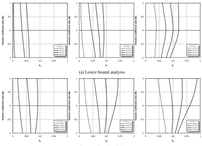
(a) Lower bound analysis
0 0.25 0.5 0.75 1
kh -1 -0.5 0 0.5 1 S e is m ic c o e ff ic ie n t ra ti o ( c ) Nc=0.10 tan=0.2 tan=0.4 tan=0.6 tan=0.8
0 0.25 0.5 0.75 1
kh -1 -0.5 0 0.5 1 S e is m ic c o e ff ic ie n t ra ti o ( c ) Nc=0.15 tan=0.2 tan=0.4 tan=0.6 tan=0.8
0 0.25 0.5 0.75 1
kh -1 -0.5 0 0.5 1 S e is m ic c o e ff ic ie n t ra ti o
(c
)
Nc=0.20 tan=0.2 tan=0.4 tan=0.6 tan=0.8
(b) Upper bound analysis
Figure 4. The relations between horizontal seismic coefficient and seismic coefficient ratio by safety number (60)
EXAMPLE
0 0.25 0.5 0.75 1
kh
-1 -0.5 0 0.5 1
S
e
is
m
ic
c
o
e
ff
ic
ie
n
t
ra
ti
o
(c
)
(a) Size of slope and Properties (b) Analysis conditions for Horizontal seismic coefficient and Seismic coefficient ratio
Figure 5. Analysis conditions of verification examples 3
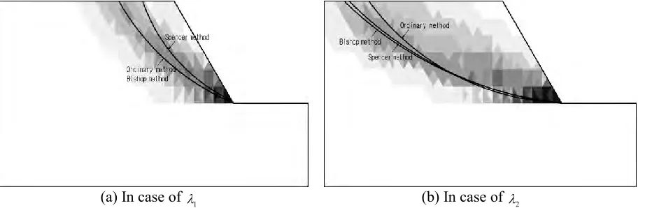
The plastic zone by upper bound analysis and the failure surface by limit equilibrium analysis are shown in a diagram and compared in Figure 6. On the lower side of the slope where plastic energy is the largest and most highly concentrated, the failure surface coincides very well. On the other hand, the failure surface is a little different on the upper side of the slope, where plastic energy is low and the plastic zone is widespread. However, the overall behavior of the slope shows a similar result.
(a) In case of 1 (b) In case of 2
Figure 6. Comparison of Plasticity energy and Failure surface by Seismic coefficient ratio
CONCLUSION
The effect of vertical inertia force is characterized by its magnitude and direction unfavorable to seismic stability of slopes. A numerical limit analysis program is developed and applied in order to investigate the effect of vertical inertia force on site-specific basis. As a result of analyses, charts for determining magnitude and unfavorable direction of vertical inertia force are proposed under various conditions of slope and earthquake loading.
ACKNOWLEDGEMENT
REFERENCES
Chang, C. J., Chen, W. F. & Yao, J. T. P., (1984), “Seismic displacement in slopes by limit analysis.”, J. Geotech. Engng, ASCE, 110(7), 860-874.