ABSTRACT
MULGRAVE, JAMI JACKSON. Bayesian Inference in Nonparanormal Graphical Models. (Under the direction of Subhashis Ghoshal).
This dissertation focuses on Bayesian inference in nonparanormal graphical models, a
nonpara-metric extension of Gaussian graphical models. We develop computational methods for learning
the structure of these models and study their theoretical properties.
In Chapter 2, we consider a Bayesian approach in the nonparanormal graphical model by putting
priors on unknown transformations through a random series based on B-splines where the
coeffi-cients are ordered to induce monotonicity. A truncated normal prior leads to partial conjugacy in
the model and is useful for posterior simulation using Gibbs sampling. On the underlying precision
matrix of the transformed variables, we consider a spike-and-slab prior and use an efficient posterior
Gibbs sampling scheme. We use the Bayesian Information Criterion to choose the hyperparameters
for the spike-and-slab prior. We present a posterior consistency result on the underlying
transfor-mation and the precision matrix. We study the numerical performance of the proposed method
through an extensive simulation study and finally apply the proposed method on a gene microarray
data set.
In Chapter 3, we continue using the random series B-spline priors on the unknown
transfor-mations of the nonparanormal graphical model, but we consider a different prior on the precision
matrix. We use a regression based formulation to construct a likelihood through the Cholesky
de-composition of the underlying precision matrix of the transformed variables and put shrinkage
priors on the regression coefficients. We apply a plug-in variational Bayesian algorithm for learning
the sparse precision matrix and compare the performance with a posterior Gibbs sampling scheme
in a simulation study. We finally apply the proposed methods to a gene expression data set.
In Chapter 4, we consider a Bayesian approach for the nonparanormal graphical model using a
rank likelihood. The rank likelihood remains invariant under monotone transformations, thereby
of the transformed variables, we continue to use the horseshoe prior on its Cholesky decomposition
and use an efficient posterior Gibbs sampling scheme. We present a posterior consistency result
on the rank-based transformation. We study the numerical performance of the proposed method
© Copyright 2018 by Jami Jackson Mulgrave
Bayesian Inference in Nonparanormal Graphical Models
by
Jami Jackson Mulgrave
A dissertation submitted to the Graduate Faculty of North Carolina State University
in partial fulfillment of the requirements for the Degree of
Doctor of Philosophy
Statistics
Raleigh, North Carolina
2018
APPROVED BY:
Alyson Wilson Alison Motsinger-Reif
Russell Wolfinger Subhashis Ghoshal
DEDICATION
BIOGRAPHY
Jami Jackson Mulgrave was born in Durham, North Carolina. She graduated from Columbia
Univer-sity with a Bachelor of Arts degree in Psychology and a concentration in the Premedical Sciences.
After graduating, she worked for five years in clinical research at Memorial Sloan-Kettering Cancer
Center. During her employment, she became interested in machine learning and data science and
the impact of those areas in health care, so she decided to apply to Ph.D. programs in Statistics. She
joined North Carolina State University to earn a Ph.D. in Statistics. She earned a Master of Statistics
degree with a concentration in statistical genetics in 2015 at North Carolina State University. She
will be joining the Department of Biomedical Informatics at Columbia University as a postdoctoral
ACKNOWLEDGEMENTS
I would like to thank Dr. Subhashis Ghoshal for his steadfast encouragement and patience
through-out the dissertation process. Dr. Ghoshal has been the best advisor that I could ever ask for. His
personality and research style is a compliment to mine and I believe that I grew into an independent
researcher from his mentoring and support. I grew to love research under his tutelage and it was
largely due to his willingness to give me room as a student to discover and solve problems.
I would also like to thank Dr. Spencer Muse for putting me on his Biostatistics and Bioinformatics
training grant. I will never forget the moment that I received the e-mail from him before I started the
graduate program in which I learned that I will be on a grant and will take biostatistics and genetics
classes and attend a statistical genetics conference. I could not believe my luck, especially since I
was already interested in healthcare analytics.
I must also thank Dr. Kimberly Weems. She was my academic advisor for the graduate program
and I was fortunate enough for an advisor such as her to review my academic background and
suggest that I take certain classes to fill in the gaps. I am so glad that I was able to develop the proper
background for the Ph.D. degree in Statistics at North Carolina State University.
I must acknowledge Dr. Monahan, Dr. Fuentes, and Dr. Shafer who were all very supportive of
me as a graduate student. I would like to thank Dr. Reneé Moore for her support and encouraging
conversations. Lastly, I would like to thank my parents who always knew that I could earn a Ph.D. in
TABLE OF CONTENTS
LIST OF FIGURES. . . vii
Chapter 1 INTRODUCTION . . . 1
1.1 Markov Properties for Undirected Graphs . . . 3
1.2 Gaussian Graphical Models . . . 4
1.3 Estimating a Sparse Precision Matrix . . . 5
1.3.1 Classical Methods . . . 5
1.3.2 Bayesian Methods . . . 6
1.4 Constructing Undirected Graphical Models using Transformed Data . . . 7
1.4.1 Nonparanormal Graphical Models . . . 8
1.4.2 Copula Gaussian Graphical Models . . . 8
1.5 Our Contribution . . . 10
Chapter 2 Bayesian Inference in Nonparanormal Graphical Models . . . 11
2.1 Introduction . . . 11
2.2 Model and Priors . . . 13
2.3 Posterior Computation . . . 20
2.3.1 Gibbs Sampling Algorithm . . . 20
2.3.2 Choice of Prior Parameters . . . 23
2.4 Posterior Consistency . . . 25
2.5 Simulation . . . 28
2.6 Real Data Application . . . 33
2.7 Proof of Consistency Theorems . . . 38
2.8 Discussion . . . 40
Chapter 3 Regression Based Bayesian Approach for Nonparanormal Graphical Models. . 42
3.1 Introduction . . . 42
3.2 Model and Priors . . . 44
3.2.1 Nonparanormal Transformation . . . 44
3.2.2 Cholesky Decomposition Reformulated as Regression Problems . . . 45
3.2.3 Sparsity Constraint . . . 46
3.3 Variational Bayes Estimation . . . 47
3.3.1 Tuning Procedure . . . 50
3.4 MCMC Estimation through Horseshoe Prior . . . 52
3.4.1 Horseshoe Prior . . . 52
3.4.2 Horseshoe Posterior . . . 53
3.5 MCMC Estimation through Bernoulli-Gaussian Prior . . . 55
3.5.1 Bernoulli-Gaussian Prior . . . 55
3.5.2 Bernoulli-Gaussian Posterior . . . 55
3.6 Thresholding . . . 57
3.7 Choice of Prior Parameters . . . 58
3.8.1 Performance Assessment . . . 62
3.9 Real Data Application . . . 66
Chapter 4 Rank Likelihood for Bayesian Nonparanormal Graphical Models . . . 70
4.1 Introduction . . . 70
4.2 Model and Priors . . . 72
4.2.1 Estimation of Transformed Variables . . . 72
4.2.2 Estimation of Inverse Correlation Matrix . . . 73
4.3 Posterior Computation . . . 74
4.4 Thresholding . . . 76
4.5 Choice of Prior Parameters . . . 77
4.6 Posterior Consistency . . . 78
4.7 Simulation Results . . . 80
4.7.1 Performance Assessment . . . 83
4.8 Real Data Application . . . 84
LIST OF FIGURES
Figure 1.1 An undirected graph. . . 2
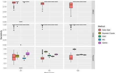
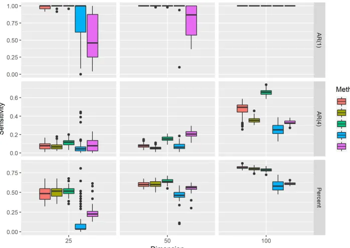
Figure 2.1 Sensitivity results. . . 33
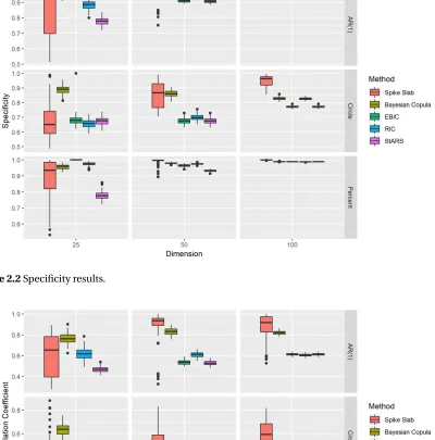
Figure 2.2 Specificity results. . . 34
Figure 2.3 Matthews correlation coefficient results. . . 34
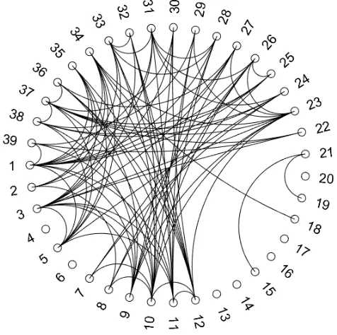
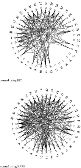
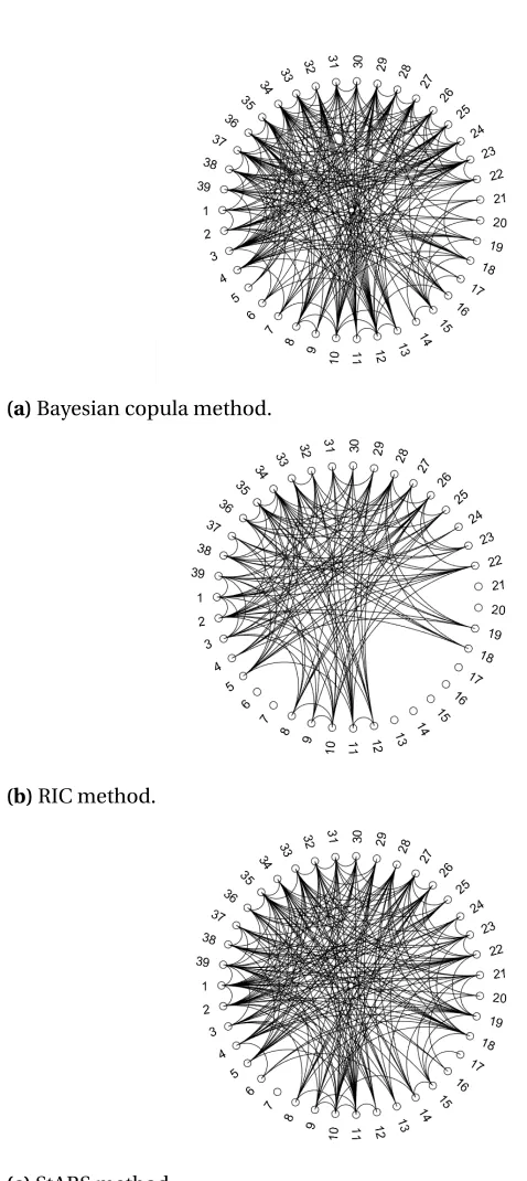
Figure 2.4 Comparison of graphical models for microarray data set. . . 36
Figure 2.5 Comparison of graphical models for microarray data set. . . 37
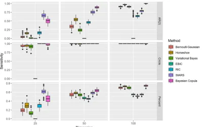
Figure 3.1 Sensitivity results. . . 64
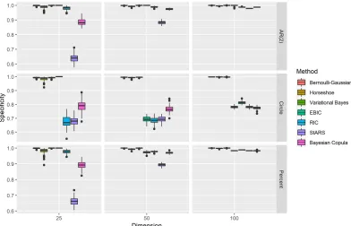
Figure 3.2 Specificity results. . . 65
Figure 3.3 Matthews correlation coefficient results. . . 65
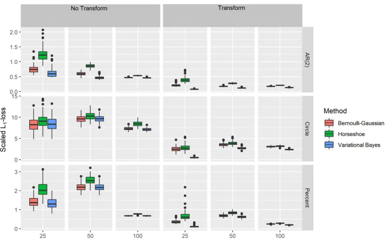
Figure 3.4 Comparison of scaledL1-loss with and without transformation. . . 66
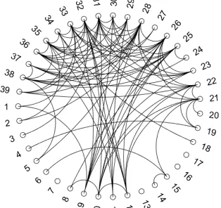
Figure 3.5 Comparison of models from proposed methods. . . 68
Figure 3.6 Comparison of models from existing methods. . . 69
Figure 4.1 Sensitivity results. . . 85
Figure 4.2 Specificity results. . . 85
Figure 4.3 Matthews correlation coefficient results. . . 86
Figure 4.4 ScaledL1-loss results. . . 86
Figure 4.5 Comparison of Rank Likelihood and B-splines methods . . . 88
CHAPTER
1
INTRODUCTION
Graphical models are probabilistic models that describe relationships between variables. A graph
G= (V,E)consists of a setV of vertices and a setE of edges between these vertices. The vertices
represent the variables in the model and the edges encode the relations. The two basic types of graphs
are directed and undirected graphs. Directed graphs represent antisymmetric relations between
variables while undirected graphs represent symmetric relations between variables. In a graphical
model, the vertices of a graph correspond to a group of random variablesX = (X1, . . . ,Xp)∼P, where
P is the probability distribution ofX. The pair(G,P)is referred to as a graphical model which has
vertex setV withpelements for each component ofXand edge setEwhich consists of ordered pairs
(d,k)where(d,k)∈ Eif there is an edge betweenXdandXk. The edge between(d,k)is excluded
fromE if and only ifXd is independent ofXk given all other variables, to be denoted byXV \{d,k}. Graphical models have been developed for complex high-dimensional problems since these models
models have been used in diverse areas such as medicine, robotics, intelligent tutors, information
retrieval, and reliability analysis.
Undirected graphical models are generally used for problems in which there is little causal
structure due to the symmetric relationships between the variables. Problems such as these include
scene object recognition (Ruiz-Sarmiento, Galindo & Gonzalez-Jimenez, 2017), protein engineering
(Thomas, Ramakrishnan & Bailey-Kellogg, 2009), and indoor tracking and navigation for
smart-phones (Xiao et al., 2015). Undirected graphical models are the main models of interest for this work.
Figure 1 is an example of an undirected graph with five variables. In this example, variablesX and
Y are independent givenZ,U, andV since there is no edge between them, and likewise,X andU
are independent givenZ,V, andY.
Figure 1.1An undirected graph.
The benefit of decomposition is that a complicated distribution on a high-dimensional domain
can be reconstructed from distributions on lower-dimensional subspaces. Conditional
indepen-dence links decompositions of distributions to graphical models. Separation in graphs is a qualitative
representation of decomposition in graphs and can be used to represent conditional independence.
For the undirected graphG with three disjoint subsets of nodesX,Y, andZ,Z separatesX andY
inG if without the nodes inZ, the nodes inX and the nodes inY are not connected (Borgelt et al.,
2009). However, it can be tedious to check for all separations of node sets in a graph to see if the
nodes are conditionally independent. Simpler criteria can be used to characterize conditional
inde-pendence structure: Markov properties of graphs. Assuming a Markov property of the distribution
variablesX1, . . . ,Xp.
1.1
Markov Properties for Undirected Graphs
Definition 1.1.1. We say thatP satisfies the pairwise Markov property with respect to the undirected graphG if for any pair of distinct vertices(j,k)∈ E/ (j6=k),
Xj ⊥Xk|XV \{j,k}.
A stronger property is the global Markov property defined below.
Definition 1.1.2. We say thatP satisfies the global Markov property with respect to the undirected graphG if for any triplet of disjoint setsA,B,C such thatC separatesAandB,
XA⊥XB|XC.
The global Markov property implies the pairwise Markov property. These two properties are
equivalent for a large class of models under a set of specific conditions detailed in Proposition 1.1.1.
Proposition 1.1.1. If the distribution P has a positive and continuous density with respect to Lebesgue measure, the global and pairwise Markov properties are equivalent.
Finally, within the class of undirected graphical models, we have the most popular model defined
below.
Definition 1.1.3. A conditional independence graph (CIG) is a graphical model(G,P), with undi-rected graphG, where the pairwise Markov property holds.
Thus, a CIG has the property: if(j,k)∈ E/ (j6=k), thenXj ⊥Xk|XV \{j,k}. WhenP is multivariate Gaussian, the converse is true as well, i.e., ifXj ⊥Xk|XV \{j,k}, then(j,k)∈ E/ .
See Bühlmann & Geer (2011) for more information on graphical models and the Markov
multivariate Gaussian, it is called a Gaussian graphical model. Gaussian graphical models are our
main area of interest.
1.2
Gaussian Graphical Models
A Gaussian graphical model (GGM) is a conditional independence graph with a multivariate
Gaus-sian distribution such that
X = (X1, . . . ,Xp)∼Np(0,Σ)
with positive definitep×pcovariance matrixΣand inverse covariance matrixΣ−1=Ω. The mean zero assumption is used to simplify the notation. The pairwise Markov property in the CIG is
equivalent to the global Markov property due to the Gaussian assumption.
A well known result is that the edges in a GGM are given by the inverse of the covariance matrix
(Lauritzen, 1996):
(j,k)and(k,j)∈ E ⇔/ Xj⊥Xk|XV \{j,k}⇔ωj,k=0,
whereΩ= ((ωj,k)). Thus, GGMs have an “if and only if” interpretation of an edge which is stronger than in CIGs.
In addition, another well-known result is that the inverse of the covariance matrix corresponds
to partial correlations (Lauritzen, 1996):
ρj,k|V \{j,k}=−
ωj,k pω
j,jωk,k
Finally, we can relate partial correlations directly to regression coefficients. Consider the
regres-sion model
Xj =βj,kXk+ X
r∈V \{j,k}
βr,jXr+εj,
(Bühlmann & Geer, 2011). Then,
βj,k=−
ωj,k
ωj,j .
Thus, we have the following equivalences for a GGM:
(j,k)and(k,j)∈ E ⇔ωj,k6=0⇔ρj,k|V \{j,k}=6 0⇔βj,k6=0.
Thus, GGMs are flexible models that can be linked to variable selection problems in regression,
particularly for high-dimension. GGMs have been used for biological networks (Wang et al., 2016),
metabolomics (Krumsiek et al., 2011), gene networks (Ma, Gong & Bohnert, 2007; Krämer, Schäfer &
Boulesteix, 2009; Ingkasuwan et al., 2012), climate networks (Zerenner et al., 2014), link prediction
(Zhang et al., 2016), and dietary pattern analysis (Iqbal et al., 2018).
1.3
Estimating a Sparse Precision Matrix
Estimating a sparse precision matrix is necessary to construct a Gaussian graphical model. Typical
estimators like the sample covariance matrix or the maximum likelihood estimator are not suitable
for problems in which the dimension can be high relative to the sample size. In addition, these
estimators are not generally sparse, so regularization is needed.
1.3.1 Classical Methods
Several techniques have been proposed in the literature to estimate sparse precision matrices. Let
Y(n×p)be the data matrix ofpvariables andnsamples such thatS=Y0Yis the sum of the products matrix. A widely used frequentist approach to estimate the precision matrix is to add an`1(lasso) penalty on the entries of the precision matrix and maximize the penalized log-likelihood,
log(det(Ω))−tr(S
over the space of positive definite matricesM+with penalty parameterρ≥0. The||Ω||1= P
1≤j,k≤p|ωj k|is the`1norm ofΩ. This approach is known as the graphical lasso (Friedman, Hastie & Tibshirani, 2008) and it can be used to simultaneously estimate the precision matrix and find
structures in the graphical model. Many algorithms have been proposed to solve this problem
(Meinshausen & Buhlmann, 2006; Yuan & Lin, 2007; Friedman, Hastie & Tibshirani, 2008; Banerjee,
El Ghaoui & d’Aspremont, 2008; d’Aspremont, Banerjee & El Ghaoui, 2008; Rothman et al., 2008;
Lu, 2009; Scheinberg, Ma & Goldfarb, 2010; Witten, Friedman & Simon, 2011; Mazumder & Hastie,
2012b). The lasso penalty has been shown to produce substantial biases, so the smoothly clipped
absolute deviation penalty and the adaptive lasso penalty have been proposed to reduce these
biases for precision matrix estimation (Fan, Feng & Wu, 2009).
1.3.2 Bayesian Methods
Bayesian methods for GGMs involve using priors on the precision matrix and priors on the graph as
well. A popular prior on a precision matrix is given by the family of G-Wishart priors (Giudici, 1999;
Roverato, 2002; Atay-Kayis, 2005; Letac & Massam, 2007; Wang & Carvalho, 2010; Dobra, Eicher &
Lenkoski, 2010; Mitsakakis, Massam & D. Escobar, 2011; Lenkoski & Dobra, 2011; Dobra, Lenkoski
& Rodriguez, 2011; Wang & Li, 2012). The G-Wishart prior is conjugate to multivariate normal
random variables and yields an explicit expression for the posterior mean. If the underlying graph
is decomposable, the normalizing constant in a G-Wishart distribution has a simple closed form
expression. In the absence of decomposability, the expression is more complex (see (Uhler, Lenkoski
& Richards, 2017)), but may be computed by simulations. Computation of the marginal likelihood,
and hence the posterior probability, of any given graph is possible with the
R
packageBDgraph
(Mohammadi & Wit, 2015; Mohammadi & Wit, 2017; Dobra & Mohammadi, 2017; Mohammadi &
Wit, 2018). However, as the number of possible graphs is huge, computing posterior probabilities
of all graphs is an impossible task for even a moderate number of nodes. Thus when learning the
graphical structure from the data, alternative mechanisms of putting priors on the entries of the
matrix is ideally a mixture of a point mass at zero and a continuous component (Wong, Carter &
Kohn, 2003; Carter, Wong & Kohn, 2011; Talluri, Baladandayuthapani & Mallick, 2014; Banerjee &
Ghosal, 2015). However, since the normalizing constants in these mixture priors are intractable
due to the positive definiteness constraint on the precision matrix, absolutely continuous priors
have been proposed. The Bayesian graphical lasso (Wang, 2012) has been developed as a Bayesian
counterpart to the graphical lasso. However, its use of a double exponential prior, which does not
have enough mass at zero, does not give a true Bayesian model for sparsity. Continuous shrinkage
priors, such as the horseshoe (Carvalho, Polson & Scott, 2010), generalized double Pareto (Armagan,
B. Dunson & Lee, 2013), Dirichet-Laplace (Bhattacharya et al., 2015), and others have been proposed
as better models of sparsity in the linear models context since these priors have infinite spikes
at zero and heavy tails. Such continuous priors have been applied to GGMs including uniform
shrinkage priors (Wang & Pillai, 2013), normal spike-and-slab priors (Wang, 2015; Peterson, Stingo &
Vannucci, 2016; Li & McCormick, 2017; Li, McCormick & Clark, 2017), Laplace spike-and-slab priors
Gan, Narisetty & Liang (2018), and the horseshoe prior (Williams et al., 2018). From a computational
point of view, continuous shrinkage priors such as the horseshoe prior (Carvalho, Polson & Scott,
2009), the Dirichlet-Laplace prior (Bhattacharya et al., 2015), and generalized double exponential
prior (Armagan, B. Dunson & Lee, 2013), bring in the effects of both a point mass and a thick tail by
a single continuous distribution with an infinite spike at zero.
1.4
Constructing Undirected Graphical Models using Transformed Data
Gaussian graphical models are flexible models used to learn relationships between continuous
variables, but the Gaussianity assumption can be restrictive in many settings. The usual course of
action is to transform the data to make it as close to normal as possible. One strategy to transform
data would be, for instance, a logarithmic transformation, but that is not the only strategy. Instead
of trying different transformations, like a logarithmic transform or square root transform, we may
instead leave the transformation functions unspecified and use a nonparametric technique. The
have been developed to use nonparametric techniques to transform the data. Once the data are
transformed, one can estimate a sparse precision matrix using the methods discussed in Section
1.3. Our main research interest is on the development of nonparanormal graphical models for
continuous data.
1.4.1 Nonparanormal Graphical Models
We consider a nonparametric extension of GGMs based on multivariate Gaussian distributions in the
high dimensional setting. A nonparametric extension of the normal distribution is the
nonparanor-mal distribution in which the random variablesX= (X1, . . . ,Xd)are replaced by some transformed random variablesf(X):= (f1(X1), . . . ,fd(Xd))and it is assumed thatf(X)has ad-variate normal distribution Nd(µ,Σ) (Liu, Lafferty & Wasserman, 2009).
Definition 1.4.1. A random vectorX= (X1, ...,Xp)has a nonparanormal distribution if there exist smooth monotone functions{fd :d =1, . . . ,p} such thatY =f(X)∼Np(µ,Σ), where f(X) = (f1(X1), . . . ,fp(Xp)). In this case we shall writeX∼NPN(µ,Σ,f).
Liu, Lafferty & Wasserman (2009) designed the nonparanormal graphical model using a
two-step estimation process in which the functionsfj were estimated first using a truncated empirical distribution function, and then the inverse covariance matrixΩ=Σ−1 was estimated using the graphical lasso applied to the transformed data. Nonparanormal graphical models have been
applied to gene regulatory networks (Jia et al., 2017) and edge detection (Jia et al., 2017).
1.4.2 Copula Gaussian Graphical Models
Nonparanormal graphical models can be constructed using a two-step statistical procedure in
which one estimates the transformation functions and then estimates the sparse precision matrix.
Gaussian copula graphical models (GCGMs) avoid the estimation of the transformation functions
by using rank-based methods to transform the data. Rank-based methods are invariant under
monotone transformations, and so can safely replace methods that estimate the transformation
for continuous data, but we differentiate nonparanormal graphical models as a type of
nonpara-metric model in which the transformation functions are being estimated and GCGMs as a type of
nonparametric model in which estimating the transformation functions is not necessary.
In the frequentist literature, nonparametric rank-based correlation coefficient estimators have
been used to achieve estimation robustness. Using the definition of a nonparanormal distribution,
we have the observed variables(x1i,x2i, . . . ,xn1)and the transformed variablesY. We can convert the observed variables to ranks denoted byri= (r1i,r2i, . . . ,rn i). Spearman’s rank correlation ˆri j is a nonparametric measure of dependence between two variables and is defined as the Pearson’s
correlation betweenriandrj (Xue & Zou, 2012). Observing thatri are the ranks of the unobserved variables, or the “oracle” variables, ˆri j is also identical to the Spearman’s rank correlation between the “oracle” variables (Xue & Zou, 2012). Thus, we can avoid estimating the transformation functions
by using the observed data. Liu et al. (2012) and Xue & Zou (2012) used Spearman’s rank correlation
and the alternative Kendall’s tau correlation to transform the data, and then estimated the sparse
precision matrix using the graphical lasso, Dantzig selector (Yuan, 2010), and CLIME (Cai, Liu & Luo,
2011). Zhao, Roeder & Liu (2014) developed a projection algorithm that theoretically guarantees
a positive semidefinite correlation matrix based on the Kendall’s tau estimator. He et al. (2017)
estimated a GCGM by simultaneous tests which control the false discovery rate.
Bayesian inference in copula models were first introduced in the regression context (Pitt, Chan
& Kohn, 2006). The authors used the covariance selection prior introduced in Wong, Carter &
Kohn (2003) for the correlation matrix. However, the marginal distributions must belong to specific
parametric families. Hoff (2007) developed a semiparametric estimation strategy using the extended
rank likelihood under a Bayesian framework in which the marginal distributions are arbitrary
and of unspecified types, thus accommodating both discrete and continuous data. The extended
rank likelihood is a likelihood function that depends on the associations between the variables
and not on the unknown marginal distributions. For continuous data, this function is equivalent
to the distribution of the multivariate ranks. The rank likelihood falls under the setup of linear
developed in the graphical model setting to construct a GCGM by Dobra & Lenkoski (2011) using
the Bayesian model averaging approach for graph identification and estimation. Dobra & Lenkoski
(2011) used a G-Wishart prior and Markov Chain Monte Carlo to estimate the sparse precision
matrix. Mohammadi et al. (2017) constructed this Bayesian GCGM similar to Dobra & Lenkoski
(2011) in order to model Dupuytren disease.
Alternative methods to estimate a sparse precision matrix for the GCGM have been proposed
in the Bayesian setting beyond the G-Wishart prior. Abegaz & Wit (2015) estimated a GCGM using
the extended rank likelihood and putting an`1-penalty on the precision matrix in an EM algorithm. More recently, Li & McCormick (2017) estimated a GCGM using the extended rank likelihood with a
normal spike-and-slab prior on the precision matrix in an expectation conditional maximization
algorithm.
1.5
Our Contribution
We present research that contributes to the Bayesian literature on nonparanormal graphical models.
Currently, there has not been a Bayesian counterpart to the nonparanormal graphical model that has
been developed. In the second chapter, we present a Bayesian nonparanormal graphical model. We
construct the random series prior using B-splines that we employ to estimate smooth transformation
functions. On the precision matrix, we consider a spike-and-slab prior. In the third chapter, we
modify our approach to estimate the sparse precision matrix by using a Cholesky decomposition of
the precision matrix and we consider two different priors, the horseshoe and Bernoulli-Gaussian
prior, as well as two estimation methods, Markov Chain Monte Carlo estimation and variational
Bayesian optimization. Continuous shrinkage priors have not been used in the context of Bayesian
Gaussian copula graphical models. In the last chapter, we use a horseshoe prior to construct a
Bayesian estimation procedure in Gaussian copula graphical models and compare its performance
CHAPTER
2
BAYESIAN INFERENCE IN
NONPARANORMAL GRAPHICAL
MODELS
2.1
Introduction
In this chapter, we develop Bayesian methods for estimating in a nonparanormal graphical model.
Chapter 1 introduced the basic ideas underlying graphical models and reviewed the definition of
nonparanormal graphical models. As discussed, Liu, Lafferty & Wasserman (2009) designed the
matrixΩ=Σ−1was estimated using the graphical lasso applied to the transformed data. Although the approach in Liu, Lafferty & Wasserman (2009) works well in many settings, their estimator for
the transformation functions is based on the empirical distribution function, which leads to an
unsmooth estimator. While the focus of this chapter is on the nonparanormal graphical model, an
alternative to the nonparanormal graphical model is the copula Gaussian graphical model (Pitt,
Chan & Kohn, 2006; Dobra & Lenkoski, 2011; Liu et al., 2012; Mohammadi & Wit, 2017) which avoids
estimation of the transformation functions by using rank-based methods to transform the observed
variables.
Bayesian approaches can naturally blend the desired smoothness in the estimate by considering
a prior on a function space that consists of smooth functions. Gaussian process priors are the most
commonly used priors on functions (Rasmussen & Williams, 2006; Choudhuri, Ghosal & Roy, 2007;
Vaart & Zanten, 2007; Lenk & Choi, 2017). Priors on function spaces have also been developed
using a finite random series of certain basis functions like trigonometric polynomials, B-splines,
or wavelets (Rivoirard & Rousseau, 2012; Jonge & Zanten, 2012; Arbel, Gayraud & Rousseau, 2013;
Shen & Ghosal, 2015). We consider a Bayesian approach using a finite random series of B-splines
prior on the underlying transformations. We choose the B-splines basis over other possible choices
because B-splines can easily accommodate restrictions on functions, such as monotonicity and
linear constraints, without compromising good approximation properties (Shen & Ghosal, 2015). In
our context, as the transformation functionsf1, . . . ,fd are increasing, imposing the monotonicity restriction through the prior is essential. This can be easily be installed through a finite random
series of B-splines by imposing the order restriction on the coefficients. By equipping the vector of
the coefficients with a multivariate normal prior truncated to the cone of ordered coordinates, the
order restriction can be imposed maintaining the conjugacy inherited from the original multivariate
normal distribution. A simple Gibbs sampler is constructed in which first, a truncated normal
prior on the transformation functions results in a truncated normal posterior distribution that is
sampled using a Hamiltonian Monte Carlo technique (Pakman & Paninski, 2014). Second, a Student
corresponding posterior distribution of the precision matrix and the edge matrix, which determines
the absence or presence of an edge in the graphical model. The underlying graphical structure can
then be constructed from the obtained edge matrix.
The chapter is organized as follows. In the next section, we specify the prior distributions for
the underlying parameters. In Section 2.3, we obtain the posterior distributions, describe the Gibbs
sampling algorithm and the tuning procedure. In Section 2.4, we provide a posterior consistency
result for the priors under consideration. In Section 2.5, we present a simulation study. In Section
2.6, we apply the method to a real data set and we provide proofs in Section 2.7. Finally, we conclude
with a discussion section.
2.2
Model and Priors
Recall Definition 1.4.1 of a nonparanormal graphical model. By assuming that the transformed
variablesf(X)are distributed as normal, the conditional independence information in the nonpara-normal model is completely contained in the parameterΩ, as in a parametric normal model. Since
the transformation functions are one-to-one, the inherent dependency structure given by the graph
for the observed variables is retained by the transformed variables. We note that any continuous
random variable can be transformed to a normal variable by a strictly increasing transformation.
However testing for high-dimensional multivariate normality is not feasible, and hence testing for
the nonparanormality assumption is not possible in high dimension, but clearly the condition is
a lot more general than multivariate normality. Instead of testing for nonparanormality, one may
assess the efficacy of the assumption by looking at the effect of the transformations. If the
trans-formation functions are linear, then assuming multivariate normality should be adequate. If the
transformation functions are non-linear, then modeling through the nonparanormal distribution
may be useful.
We put prior distributions on the unknown transformation functions through a random series
based on B-splines. The coefficients are ordered to induce monotonicity, and the smoothness is
Cubic splines, which are B-splines of degree 4, are used in this chapter. The resulting posterior means
of the coefficients give rise to a monotone smooth Bayes estimate of the underlying transformations.
Thus the smooth monotone functions that we use to estimate the true transformation functions
are assumed to be multivariate normal,
f(X) =
J X
j=1
θjBj(X)∼Np(µ,Ω−1), (2.1) wheref is ap-vector of functions,X is ann×p matrix, andθj is ap-vector; hereBj(·)are the B-spline basis functions,θj are the associated coefficients in the expansion of the function, andJ is the number of B-spline basis functions used in the expansion. These transformed variablesf(X)
are subsequently used to estimate the sparse precision matrix and hence in structure learning.
In the next part, we discuss the prior on the coefficients in more detail.
• Prior on the B-spline coefficients
First, we temporarily disregard the monotonicity issue and put a normal prior on the
co-efficients of the B-splines,θ ∼NJ(ζ,σ2I), whereσ2 is some positive constant,ζ is some vector of constants, andI is the identity matrix. A normal prior is convenient as it leads to conjugacy. However, apart from monotonicity of the transformations, we also need to address
identifiability since unknownµandΣallow flexibility in the location and the scale of the transformation so that the distribution off(X)can be multivariate normal for many different choices off. The easiest way to address identifiability is to standardize the transformations by settingµ=0and the diagonal entries ofΣto 1. However, then it will be more difficult to put a prior on sparseΩcomplying with the restriction on the diagonal entries ofΣbecause
of the constraintΣ=Ω−1. Hence it is easier to keepµandΩfree and impose restrictions on the locations and the scales of the transformation functions fd,d =1, . . . ,p. There are different ways to impose constraints on the locations and scales offd. One can impose some location and scale restrictions on the corresponding B-spline coefficients, for instance, by
making the mean ¯θd=J−1 PJ
j=1θd j =0 and the variance ¯θd=J−1 PJ
the prior distribution forθd,d =1, . . . ,p, will have to be conditioned on these restrictions. The non-linearity of the variance restriction makes the prior less tractable. In order to obtain
a conjugate normal prior, we instead consider the following two linear constraints on the
coefficients through function values of the transformations:
0=fd(1/2) = J X
j=1
θd jBj(1/2), (2.2)
1=fd(3/4)−fd(1/4) = J X
j=1
θd j[Bj(3/4)−Bj(1/4)]. (2.3)
It may be noted that, as only a few B-spline functions are non-zero at any given point, the
restrictions (2.2) and (2.3) involve only a fewθjs. More specifically, as the degree of B-splines used in this paper is 4, the first equation involves only 4 coefficients and the second only 8, no
matter how largeJ is.
The linear constraints can be written in matrix form as
Aθ=c, (2.4)
where
A=
B1(1/2) B2(1/2) · · · BJ(1/2)
B1(3/4)−B1(1/4) B2(3/4)−B2(1/4) · · · BJ(3/4)−BJ(1/4)
(2.5)
andc= (0, 1)0.
Using conditional normal distribution theory, the resulting prior on the coefficientsθis
where the prior mean and variance are
ξ=ζ+A0(AA0)−1(c−Aζ) (2.6) Γ=σ2[I
−A0(AA0)−1A]. (2.7)
However, the prior dispersion matrixΓis singular due to the two linear constraints, resulting
in a lack of Lebesgue density for the prior distribution onRJ. Thus, we work with a dimension reduced coefficient vector by removing two coefficients to ensure that we have a Lebesgue
density onRJ−2for the remaining components. Suppose we remove the last two coefficients. Then, the reduced vector of basis coefficients is ¯θd= [θd,1,θd,2, ...,θd,J−2]. Then we can solve forθd,J−1andθd,J usingAθ=cto obtain,
θd,J−1
θd,J
=
ad,1 ad,2 · · · ad,J−2 bd,1 bd,2 · · · bd,J−2
×θ¯d+ ad,0 bd,0 (2.8)
wheread,0, . . . ,ad,J−2,bd,0, . . . ,bd,J−2are the corresponding constants. In matrix form, we have
θd,J−1
θd,J
=Wdθ¯d+qd, (2.9)
whereWd=
ad,1 ad,2 · · · ad,J−2
bd,1 bd,2 · · · bd,J−2
andqd= ad,0 bd,0 .
Then the resulting prior for the coefficients for each predictor is,
¯
θ|{Aθ=c} ∼NJ−2(ξ¯, ¯Γ), (2.10) where the reduction is denoted with a bar.
Finally, we impose the monotonicity constraint on the coefficients, which is equivalent with
F θ>0, whereF is(J−1)×J, F =
−1 1 0 · · · 0 0
0 −1 1 · · · 0 0
· · ·
0 0 0 · · · −1 1 . (2.11)
Due to the two linear constraints, the monotonicity constraint reduces to
¯
Fθ¯+g¯>0, (2.12)
where ¯F is the(J−1)×(J−2)matrix,
¯ F=
−1 1 0 · · · 0 0
0 −1 1 · · · 0 0
· · ·
0 0 0 · · · −1 1
a1 a2 a3 · · · aJ−3 (aJ−2−1) (b1−a2) (b2−a2) (b3−a3) · · · (bJ−3−aJ−3) (bJ−2−aJ−2)
(2.13)
and ¯gis the constant(J −2)-vector, ¯g= (0, 0, 0, . . . ,a0,(b0−a0))0.
The final prior on the coefficients is given by a truncated normal prior distribution
¯
θ|{Aθ=c} ∼TNJ−2(ξ¯, ¯Γ,T), (2.14) whereT ={θ¯: ¯Fθ¯+g¯>0}, and the Np(µ,Σ)-distribution restricted on a setT is denoted by TNp(µ,Σ,T). The conjugacy property of the prior distribution is preserved by the truncation. Instead of the simplifying example of solving for the last two coefficients, we use a more
solve for any two coefficients in terms of the remaining coefficients. In particular, for the first
row of the linear constraints matrixAgiven by (2.5), we find the first column with a nonzero element. Then, for the second row of the linear constraints matrix, we find the first column
with a nonzero element that is not the same as the column selected from the first row. We use
the indices from those two columns to select the two coefficients that will be removed from
the dimension in order to find ¯θ, ¯F, and ¯g.
Although any choice ofζ is admissible, the prior can put a substantial probability of the truncation setT ={θ¯: ¯Fθ¯+g¯>0}only when the original mean vectorζ has increasing components. A simple choice ofζinvolving only two hyperparameters is given by
ζj =ν+τΦ−1
j−0.375
J −0.75+1
, j=1, . . .J, (2.15)
whereνis a constant,τis a positive constant, andΦ−1is the inverse of the cumulative distribu-tion funcdistribu-tion (i.e. the quantile funcdistribu-tion) of the standard normal distribudistribu-tion. The motivadistribu-tion
for the choice comes from imagining that the prior distribution of eachθj as N(ν,τ2)before the ordering is imposed, and hence the expectations of the order statistics of N(ν,τ2)may be considered as good choices for their means. The expressions in (2.15) give reasonable
approximation of these expectations. Similar expressionsΦ−1(j/(J+1))appear for the score function of locally most powerful rank tests against normal alternatives (see Hájek, Šidák & Sen
(1999)). Royston (1982) described the expressionΦ−1((j−0.375)/(J −0.75+1)), j=1, . . . ,J, as a more accurate approximation for the expected values of standard normal order statistics
than the expressionΦ−1(j/(J +1))used in rank tests.
• Prior on the mean
For each predictor, we put an improper uniform priorp(µ) =Qpd=1pd(µd)∝1 onµ. • Prior on the precision matrix
estimate a sparse precision matrix, but replace the normal by a Student t-distribution
spike-and-slab prior, following Scheipl, Fahrmeir & Kneib (2012). Letτ2d,k be the slab variance andc0τ2d,k be the spike variance. The spike scalec0is assumed to be very small and given. Having a continuous spike instead of a point mass at zero is more convenient since it admits
density; see Wang (2015). Unlike in Wang (2015), we estimate the sparse precision matrix by
allowing the spike-and-slab variances and probability to be random with an inverse-gamma
prior to lead to a Student t-distribution for the slabs. The diagonal entries ofΩare given an
exponential distribution with rate parameterλ/2 for someλ >0. We introduce a symmetric
matrix of latent binary variablesL= ((ld,k))with binary entries to represent the edge matrix. The entriesld,k,d<k, are assumed to be independent withπdenoting the probability of 1, i.e. the probability of an edge. Let N(·|·,·)and Exp(·|·)respectively stand for the densities of the
normal and exponential distributions. Letη= (τ2d,k,π,d<k,λ). LetM+stand for the space of positive definite matrices andvd,k2 =ld,kτ2d,k+c0τ2d,k(1−ld,k). The joint prior forΩ= ((ωd,k)) andLis then obtained as
p(Ω,L|η)∝Y d<k
N(ωd,k|0,vd,k2 ) Y
d
{Exp(ωd,d|λ/2)} Y
d<k
πld,k(1−π)ld,k1
Ω∈M+. (2.16)
The prior forη= (τ2d,k,π,d <k,λ)are given by, independently of each other,
π∼Be(1, 10), τ2d,k∼IG(b0,b1), (2.17)
where Be stands for the beta distribution and IG for the inverse-gamma distribution. The value
ofλcontrols the distribution of the diagonal elements ofΩ. We useλ=1 under similar
rea-soning to Wang (2015), because it assigns considerable probability to the region of reasonable
values of the diagonal elements. We set the shape parameters of the beta distribution to 1 and
10 to set the prior probability of sparsity to about 10%. See Scheipl, Fahrmeir & Kneib (2012)
for more details regarding the spike-and-slab prior based on a mixture of inverse gamma
2.3
Posterior Computation
The full posterior distribution is
p(θ,Ω,L,µ|X) ∝ (detΩ)n/2exp −1 2
n X
i=1
(θ0B(Xi)−µ)0Ω(θ0B(Xi)−µ)
× p Y
d=1
pd(θd)
p Y
d=1
p(µd)×p(Ω,L)1{F θ>0}, (2.18)
whereB(x) = ((Bj(xd))), the prior on the B-spline coefficients ispd(θd), the prior on the means is
p(µd), and the joint prior on the sparse precision matrix and the edge matrix isp(Ω,L). Here, the likelihood is constructed from the working assumption thatPJj=1θjBj(X)∼Np(µ,Ω−1).
The joint posteriors are standard and so they are not derived. They can be evaluated in the
following Gibbs sampling algorithm.
2.3.1 Gibbs Sampling Algorithm
1. For everyd=1, . . . ,p, sample the B-spline coefficients as follows.
(a) Since we can reduce the number of coefficients by two, the basis functions for these two
coefficients can be represented as
h
BJ−1(Xi) BJ(Xi) i
θd,J−1
θd J
=B∗θd∗ =B∗(Wdθ¯d+qd), where the∗is used to denote the two-dimensional vectorsB∗andθ∗d. SettingYd= (
PJ
j=1θd jBj(Xi d),d=1, . . . ,p,i=1, . . . ,n), the joint posterior for the B-spline coefficients is a truncated normal, with density
p(θ¯1, . . . , ¯θp|Ω,µ,Y)∝(detΩ)n/2exp − 1 2
n X
i=1
(Yi−µ)0Ω(Yi−µ)
However, this truncated multivariate normal distribution isp×(J−2)dimensional, so we
sample it using the following conditional normals in a Markov chain,
p(θ¯d|Y, ¯θ{1,...,p}\d,µ,Ω)∝exp
−1 2θ¯
0 d 1 λ2 d n X
i=1
(B¯ +B∗W
d)0(B¯ +B∗Wd) +Γ¯− 1 ¯
θd +¯
ξΓ¯−1− 1
λ2 d
n X
i=1
(B∗qd−δd,i)0(B¯+B∗Wd) θ¯d
1{F¯dθ¯d+g¯d>0},
where, using the conditional normal theory,
δd,i=µd+ X
e∈(1:p\d) (−ωd,e
ωd,d
)(Yi,e−µe)
andλ2d=1/ωd,d.
Samples from the truncated conditional normal posterior distributions for the B-spline
coefficients are obtained using the exact Hamiltonian Monte Carlo algorithm (exact HMC)
(Pakman & Paninski, 2014). Each iteration of the exact HMC results in a transition kernel
which leaves the target distribution invariant and the Metropolis acceptance probability
equal to 1. The exact HMC within Gibbs is like Metropolis within Gibbs and hence is a
valid algorithm to sample from the joint density.
2. Obtain the centered transformed variables:
(a) ComputeYi d=PJ
j=1θd jBj(Xi d); (b) Sampleµ|(Y,Ω)∼Np(Y¯,n1Ω−1); (c) FindZi d=
PJ
j=1θd jBj(Xi d)−µd=Yi d−µd. 3. The posterior density ofΩgivenLis
p(Ω|Z,L,τ2,λ)∝(detΩ)n/2exp−1 2tr(SΩ)
Y
d<k
exp −ω 2 d,k 2vd,k2
p Y
d=1
exp −λ 2ωd,d
,
For everyd =1, . . . ,p, sample each column vector ofΩandLusing the following partitions as described in Wang (2015):
• DenoteV = ((vd,k2 ))to be thep×p symmetric matrix with zeros in the diagonal and (vd2,k=ld,kτ2d,k+c0τ2d,k(1−ld,k):d<k)in the upper diagonal entries. Similarly, denote
T = ((τ2d,k))andΠ= ((πd,k))to bep×p symmetric matrices with zeros in the diagonal and(τ2d,k:d<k)and(πd,k:d<k)in the upper diagonal entries, respectively.
• Without loss of generality, partitionΩ,S,L,V,T, andΠby focusing on the last column and row:
Ω=
Ω11 ω12 ω0
12 ω22
, S=
S11 s12 s0
12 s22
, L=
L11 l12 l0
12 l22
,
V =
V11 v12 v0
12 0
, T =
T11 τ12 τ0 12 0 , Π=
Π11 π12 π0
12 0
.
• To sample a column vector ofΩ, use the following change of variables:
(ω12,ω22)7→(u=ω12,v=ω22−ω012Ω−111ω12). Then the full conditionals are given by
(u|·)∼N(−Cs12,C),(v|∗)∼Ga n 2 +1,
s22+λ 2
,
whereC={(s22+λ)Ω11−1+diag(v−121)}−1, and Ga stands for the gamma distribution. • To sample the corresponding off-diagonal column vector of the edge-inclusion indexes
ld k,d,k=1, . . . ,p,d<k, since theld,kare independent Bernoulli, we sample according to the probability
P(ld k=1|·) =
φ(ωd k|0,τ2d k)πd k
whereφstands for the normal density function.
• Updateτ2d k,d,k =1, . . . ,p,d<k, based on the off-diagonal column vectorsωd k and
ld k, using the relations
(τ2
d k|·)∼IG b0+ 1 2,b1+
ω2 d k 2 (ld k+
1−ld k
c0 )
.
• Updateπ,d,k=1, . . . ,p,d<k, based on the off-diagonal entryld k,
(π|·)∼Be(1+X d<k
1{ld k =1}, 10+ X
d<k
1{ld k=0}).
These steps are repeated until convergence.
2.3.2 Choice of Prior Parameters
We use a model selection criterion to determine the optimal number of basis functions pre-MCMC.
Sampling methods that involve putting a prior on the number of basis functions, such as reversible
jump Monte Carlo, are computationally complicated. We calculate the Akaike Information Criterion
(AIC) for different numbers of basis functions and choose the number of basis functions that
corresponded to the lowest AIC. The AIC is determined by minimizing the negative log-likelihood,
−2l(θd), respect to the basis coefficients subject to the linear and monotonicity constraints. The AIC is preferred here as the true transform does not belong to the set of splines and hence correct model
selection is not the goal, but minimizing estimated estimation error is, which is provided by the
model with the lowest AIC. The lowest AIC was found between a grid of four and 100 basis functions
by doing a search in which the lowest AIC was chosen when the next ten values were larger than
the current value in the search, since the AIC should approximately be a U-shaped curve due to
number of basis functions,J,
−2l(θd) =nlogσ2d+ 1
σ2 d
n X
i=1 XJ
j=1
θd jBj(Xi d)−µd 2
. (2.19)
After plugging in the maximum likelihood estimators (MLEs) ofµd andσd and making the substitutionZi d =Bj(Xi d)−n−1Pn
m=1Bj(Xm d), minimizing the−2l(θd)results in the following problem,
minimize θd
nlog(θd0Z0Zθd), subject toF θd>0,Aθd=c. (2.20) This problem can be equivalently solved using the quadratic programming function in MATLAB
Optimization Toolbox:
minimize θd
1 2θ
0
dZ0Zθd, subject toF θd>0,Aθd=c. (2.21) For numerical stability, the monotonicity constraint was changed toFθd≥10−4. Finally, after plugging in the solution of the quadratic programming problem ˆθd, the final number of basis functions is chosen by selecting the numberJ that minimized the AIC
AIC=−2l(θˆd) +2J =nlog(θˆ0dZ0Zθˆd) +2J.
There is some dependence on the choice of hyperparameters. We use a model selection criterion
to determine the hyperparameters,b0andb1, for inverse gamma distributions for((τ2d k))and to determine the constant value for the spike scale,c0, after the MCMC sampling. Inspired by Dahl, Roychowdhury & Vandenberghe (2005), we solve a convex optimization problem in order to use the
Bayesian Information Criterion (BIC). First, we find the Bayes estimate of the inverse covariance
matrix, ˆΩBayes. The Bayes estimate is defined as ˆΩ=E(Ω|Z). We find the average of the transformed variables, ¯Z=M−1PM
estimate of the inverse covariance matrix, ˆΩMLE:
minimize
Ω −nlog detΩ+tr(ΩS), subject toC(Ω),ˆ (2.22)
whereC represents the elements of ˆΩthat are zero and nonzero, and they are determined by the
zeros of the estimated edge matrix from the MCMC. The estimated edge matrix from the MCMC
sampler will be described in more detail in Section 2.5. This constrained optimization problem was
implemented as an unconstrained optimization problem, as described in Dahl, Roychowdhury &
Vandenberghe (2005).
Finally, we calculate BIC = −2l(ΩMLEˆ ) +klogn, wherek = #C(Ω)ˆ , the sum of the number
of diagonal elements and the number of edges in the estimated edge matrix, and−l(ΩMLE) =ˆ
−nlog det ˆΩMLE+tr(ΩMLEˆ S).
We select the combination of hyperparameters,b0,b1,c0, that results in the smallest BIC.
2.4
Posterior Consistency
Posterior consistency is a fundamental way of validating a Bayesian method using a frequentist
yardstick in the large sample setting, and is of interest to both frequentists and Bayesians; for a
thorough account of posterior consistency, see Ghosal & Vaart (2017). In Gaussian graphical models,
using point mass spike-and-slab priors, Banerjee & Ghosal (2015) showed that the posterior forΩis
consistent in the high-dimensional setting provided that(p+s)(logp)/n→0, wheres stands for the
number of non-zero off-diagonal entries of the trueΩ. With a slight modification of the arguments,
it follows that the result extends to continuous spike-and-slab priors provided that the spike scalec0 is sufficiently small with increasingp. In the nonparanormal model, the main complicating factor
comes from the unknown transformationsf1, . . . ,fp, since the rest will then be as in a Gaussian graphical model. Below we argue that these transformations may be estimated consistently in an
appropriate sense.
from the marginal likelihood for each component. Thus the problem of posterior consistency for
fd can be generically described as follows. For brevity, we drop the indexd. Consider the model
Y =f(X)∼N(µ,σ2), wheref is a continuously differentiable, strictly monotone increasing trans-formation from(0, 1)toR. Clearly, this model is not identifiable and hence consistent estimation is
not possible in the usual sense. Identifiability can be ensured by settingµ=0 andσ=1, but the
procedure followed in this paper instead puts constraints onf:f(1/2) =0 andf(3/4)−f(1/4) =1.
We shall show that the posterior forf is consistent under this set of constraints.
As the function f is necessarily unbounded near 0 and 1 to ensure thatf(X)is normally
dis-tributed, which is a distribution with unbounded support, it is clear that uniform posterior
consis-tency forf is not possible. We shall therefore consider the notion of uniform convergence on a
com-pact subset of(0, 1): for a fixedδ >0, the pseudo-metric to consider isd(f1,f2) =sup{|f1(x)−f2(x)|:
δ≤x≤1−δ}. Even then, the usual posterior distribution may be highly impacted by observations
near 0 or 1, so we actually study a modified posterior distribution, based on observations falling
within the given fixed compact subset[δ, 1−δ]of(0, 1), withδ <1/4, to be described below.
Letf0be the true transformation function, which is assumed to be continuously differentiable and strictly monotone increasing and complying with the constraints f0(1/2) =0 and f0(3/4)−
f0(1/4) =1. Letµ0andσ0>0 be respectively the true values ofµandσ. Note that the cumulative distribution function (c.d.f.) ofX is given byF(x) =P(X ≤x) =P(f(X)≤f(x)) =Φ((f(x)−µ)/σ)
and the corresponding true c.d.f. isF0(x) =Φ((f0(x)−µ0)/σ0), whereΦstands for the c.d.f. of the standard normal distribution.
Considerni.i.d. observationsX1, . . . ,Xn from the true distribution. Letn∗be the number of observations falling in[δ, 1−δ],n∗
−the number of observations falling belowδandn+∗ the number of
observations falling above 1−δ. LetX∗
1, . . . ,Xn∗∗be the observations falling in[δ, 1−δ]. The posterior consistency is based on the posterior given these complying observationsX∗
1, . . . ,Xn∗∗, and the counts (n−∗,n+∗).
Observe thatπ−:=P(X < δ) =F(δ)andπ+:=P(X >1−δ) =1−F(1−δ). Thenn−∗∼Bin(n,π−)
be the true value of(π−,π+). Then we have the identity
F(x) =π−+ (1−π+−π−)F∗(x), F0(x) =π−0+ (1−π+0−π−0)F0∗(x) (2.23)
for allx∈[δ, 1−δ].
Thus we have
f(x) =µ+σΦ−1(F(x)), f0(x) =µ0+σ0Φ−1(F0(x)). (2.24)
We note that the posterior distributions of the quantitiesπ−andπ+can be obtained based on
the countsn∗
−andn+∗ respectively. In particular, using a Dirichlet prior on the probability vector (π−,π+, 1−π−−π+), we have consistency for the posterior distribution of(π−,π+)at(π−
0,π+0). We shall assume that the posterior distribution of(π−,π+)is consistent. Note that the truncated observations
alone do not lead to a posterior distribution for(π−,π+).
The modification in the posterior distribution ofµ,σandf that we consider can be described as
follows. Using the given prior on(µ,σ,f)and the truncated observationsX1∗, . . . ,Xn∗∗, we obtain the induced posterior distribution ofF∗, while we obtain the posterior distribution on(π−,π+)directly
conditioning on(n∗
−,n+∗). Then the posterior distribution of{F(x):x∈[δ, 1−δ]}is induced from
(2.23). Finally the modified posterior distribution of(µ,σ,f)is induced from the relations
σ=1/(Φ−1(F(3/4))−Φ−1(F(1/4))), µ=− Φ
−1(F(1/2))
Φ−1(F(3/4))−Φ−1(F(1/4)), (2.25)
and (2.24) in view of the restrictions f(1/2) =0 andf(3/4)−f(1/4) =1. The corresponding true
values satisfy the analogous relations
σ0=1/(Φ−1(F0(3/4))−Φ−1(F0(1/4))), µ0=−
Φ−1(F0(1/2))
Φ−1(F0(3/4))−Φ−1(F0(1/4)). (2.26)
The following theorem on posterior consistency refers to this modified posterior distribution
rather than the original posterior distribution of(µ,σ,f).
independently, the priorΠfor f satisfies the condition that
Π(f :d(f,f0)< ε,d(f0,f00)< ε)>0for everyε >0. (2.27)
Then for anyε >0,
Π(|µ−µ0|< ε,|σ−σ0|< ε,d(f,f0)< ε|X1∗, . . . ,Xn∗∗,n−∗,n+∗)→1a.s. (2.28)
The condition on the prior for the transformationf is satisfied by the truncated normal prior
de-scribed in Section 2.2, and hence the transformationf (as well as the mean and variance parameters
µandσ2) are consistently estimated by the posterior, as shown in the following corollary.
Corollary 1. Let the prior on f be described by f =PJ
j=1θjBj, where the prior for J has infinite
support andθ= (θ1, . . . ,θJ)is given a truncated normal prior as described in Section 2.2. Then for
anyε >0,Π(f :d(f,f0)< ε,d(f0,f00)< ε)>0and hence(2.28)holds.
2.5
Simulation
We conduct a simulation study to assess the performance of the Bayesian approach to graphical
structure learning in nonparanormal graphical models. The unobserved random variables,Y1, . . . ,Yp, are simulated from a multivariate normal distribution such thatYi1, . . . ,Yi p
i.i.d.
∼ Np(µ,Ω−1)fori= 1, . . . ,n. The meansµare selected from an equally spaced grid between 1 and 2 with lengthp. We consider nine different combinations ofn,p, and sparsity forΩ:
• p=25,n=50, sparsity=10% non-zero entries in the off-diagonals
• p=50,n=150, sparsity=5% non-zero entries in the off-diagonals
• p=100,n=500, sparsity=2% non-zero entries in the off-diagonals
• p=50,n=150, AR(1) model
• p=100,n=500, AR(1) model
• p=25,n=50, circle model
• p=50,n=150, circle model
• p=100,n=500, circle model
where the circle model and the AR(1) model are described by the relations
• Circle model:ωi i=2,ωi,i−1=ωi−1,i=1, andω1,p=ωp,1=0.9
• AR(1) model:ω11=ωp p=1.9608,ωi i=2.9216 andωi,i−1=ωi−1,i=−1.3725.
The sparsity levels forΩare computed using lower triangular matrices that have diagonal entries
that are Gaussian distributed withµdiag=1 andσdiag=0.1, and non-zero off-diagonal entries that are Gaussian distributed withµ\diag=0 andσ\diag=1. Since these are lower triangular matrices, we are ensured to have positive definite matrices.
The hyperparameters for the prior are chosen to beν=1,τ=0.5, andσ2=1. The observed variablesX= (X1, . . . ,Xp)are constructed from the simulated unobserved variablesY1, . . . ,Yp. The functions used to construct the observed variables are four c.d.f.s and the power function evaluated
at the simulated unobserved variablesY1, . . . ,Yp. The four c.d.f.s are: normal, logistic, extreme value, and stable. The power function isXd = [Φ(Yd)]1/m,d =1, . . . ,p, wherem is an integer between 1 and 5. We could choose any value for the parameters, but for computational ease, we use the
maximum likelihood estimates of the parameters with the
mle
function in MATLAB. Any valuesfor the parameters could be chosen for the c.d.f.s. We choose the values of the parameters for each
of the c.d.f.s to be the maximum likelihood estimates for the parameters of the corresponding
distributions (normal, logistic, extreme value, and stable), using the variablesY1, . . . ,Yp.
The initial B-spline coefficient values for the exact HMC algorithm are constructed as follows.