Auxiliary Bootstrap Methods.

(1)

ABSTRACT

FERGUSON, BRADLEY THOMAS. Auxiliary Bootstrap Methods. (Under the direction of Eric Laber and Len Stefanski.)

(2)

(3)

Auxiliary Bootstrap Methods

by

Bradley Thomas Ferguson

A dissertation submitted to the Graduate Faculty of North Carolina State University

in partial fulfillment of the requirements for the Degree of

Doctor of Philosophy

Statistics

Raleigh, North Carolina 2018

APPROVED BY:

Eric Laber

Co-chair of Advisory Committee

Len Stefanski

Co-chair of Advisory Committee

Brian Reich Dennis Boos

(4)

DEDICATION

I dedicate my dissertation work to my parents, my children, and my wife.

At a young age my parents instilled values of hard work and constantly told me to pursue my goals. My mother in particular always told me that I could achieve whatever I wanted to in life. She was my greatest cheerleader growing up and I am forever grateful for this.

I dedicate this to my children, Thomas, Kate, and Lucy. They remind me everyday how beautiful life can be and have been a constant source of joy throughout this research process.

(5)

ACKNOWLEDGEMENTS

I wish to thank my committee members who were more than generous with their expertise and precious time. A special thanks to Dr. Eric Laber and Dr. Len Stefanski for their countless hours of reflecting, reading, encouraging, and most of all patience throughout the entire process. Thank you Dr. Brian Reich, Dr. Dennis Boos, and Dr. James Bartlett for agreeing to serve on my committee.

I would like to acknowledge and thank the North Carolina State Statistics Department for allowing me to conduct my research and providing any assistance requested. Special thanks goes to the instructors I had who helped make statistics accessible and interesting.

I would also like to acknowledge my managers at Quintiles, Dr. Valerii Fedorov and Dr. Russell Reeves who were generous in giving me time off to work on parts of my dissertation. The same goes for my current manager at DOMO, Chris Error, who has been completely supportive of finishing my PhD. I must also acknowledge Carter Rees, my main co-worker at DOMO who provided assistance with performing some simulations on Amazon AWS.

Additionally I must also acknowledge the faculty in the Brigham Young University Statis-tics Department, particularly Dr. Natalie Blades, Dr. Shane Reese, and Dr. Gilbert Fellingham. They provided crucial guidance early on in my career and encouraged me to pursue a PhD. I would be remiss if I didn’t also acknowledge Peter Dotson who provided invaluable computa-tional resources that I was able to use in the final stages of my dissertation.

(6)

TABLE OF CONTENTS

LIST OF TABLES . . . vi

LIST OF FIGURES . . . vii

Chapter 1 Introduction . . . 1

1.1 Introduction . . . 1

Chapter 2 Review of Auxiliary Quantile Estimators . . . 3

2.2 Methods . . . 4

2.2.1 Design-based estimators . . . 5

2.2.2 Model-based estimators . . . 9

2.2.3 Model-assisted estimators . . . 11

2.3 Simulation study . . . 18

2.3.1 Results . . . 20

2.4 Conclusion . . . 32

Chapter 3 R Package for Auxiliary Quantile Estimation . . . 36

3.2 Auxiliary quantile estimators . . . 37

3.2.1 Design-based estimators . . . 38

3.2.2 Model-based estimators . . . 39

3.2.3 Model-assisted generalized difference estimators . . . 40

3.2.4 Model-assisted calibration estimators . . . 41

3.3 Using the package . . . 43

3.3.1 Preparing the data . . . 43

3.3.2 Sample code for evaluating auxiliary estimators . . . 43

3.4 Conclusion . . . 47

Chapter 4 Auxiliary Bootstrap Methods . . . 48

4.2 Auxiliary bootstrap . . . 48

4.2.1 Auxiliary quantile estimator . . . 49

4.2.2 Auxiliary mean estimator . . . 50

4.2.3 Auxiliary variance estimator . . . 50

4.2.4 Choosing the number of surrogates . . . 51

4.2.5 Choosing which surrogates to label . . . 53

4.3 Proof of concept simulations . . . 54

4.3.1 Model . . . 54

4.3.2 Simulation design . . . 54

4.3.3 Results . . . 54

4.4 Simulation experiments . . . 55

(7)

4.4.2 Geospatial weather model . . . 60

4.5 Discussion . . . 62

Chapter 5 Conclusion . . . 64

References. . . 66

Appendix . . . 71

Appendix A Additional Results . . . 72

(8)

LIST OF TABLES

Table 2.1 Two-way classification of the eventsy≤Qy(α) andx≤Qx(α) in the population. 9 Table 2.2 MASE values (×102_{) and corresponding standard deviations for the}

design-based estimators with n = 100 and σ = 0.1. The smallest MASE values for

each generative model arebolded. . . 22

Table 2.3 MASE values (×102_{) and corresponding standard deviations for the} model-based estimators with n = 100 and σ = 0.1. The smallest MASE values for each generative model arebolded. . . 24

Table 2.4 MASE values (×102_{) and corresponding standard deviations for the} gener-alized difference estimators with n = 100 and σ = 0.1. The smallest MASE values for each generative model are bolded. . . 25

Table 2.5 MASE values (×102) and corresponding standard deviations for the calibra-tion estimators withn= 100 andσ= 0.1. The smallest MASE values for each generative model are bolded. . . 29

Table 3.1 Description of variables needed for data. . . 43

Table 3.2 Description of variables needed for GetModelCD Q. . . 45

(9)

LIST OF FIGURES

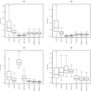
Figure 2.1 Finite populations of sizeN = 2000 generated from models 1-4 with σ= 0.1 (left) andσ = 0.3 (right). . . 21 Figure 2.2 Boxplots of ASE values (×102) for the design-based estimators from models

1-4 with n= 100 andσ= 0.1 under SRS. . . 22 Figure 2.3 Boxplots of ASE values (×102_{) for the design-based estimators from models}

1-4 with n= 100 andσ= 0.1 under Poisson sampling. . . 23 Figure 2.4 Boxplots of ASE values (×102) for the model-based estimators from models

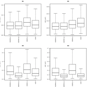
1-4 with n= 100 andσ= 0.1 under SRS. . . 25 Figure 2.5 Boxplots of ASE values (×102) for the model-based estimators from models

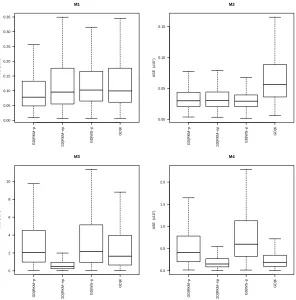
1-4 with n= 100 andσ= 0.1 under Poisson sampling. . . 26 Figure 2.6 Boxplots of ASE values (×102) for the generalized difference estimators from

models 1-4 with n= 100 andσ = 0.1 under SRS. . . 27 Figure 2.7 Boxplots of ASE values (×102) for the generalized difference estimators from

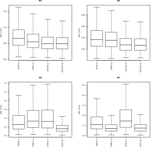
models 1-4 with n= 100 andσ = 0.1 under Poisson. . . 28 Figure 2.8 Boxplots of ASE values (×102) for the calibration estimators from models

1-4 with n= 100 andσ= 0.1 under SRS . . . 30 Figure 2.9 Boxplots of ASE values (×102) for the calibration estimators from models

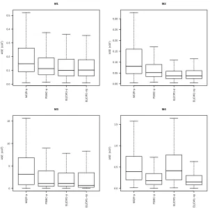
1-4 with n= 100 andσ= 0.1 under Poisson sampling. . . 31 Figure 2.10 Boxplots of ASE values (×102) from models 1-4 with n= 100 and σ = 0.1

under SRS . . . 32 Figure 2.11 Boxplots of ASE values (×102) from models 1-4 with n= 100 and σ = 0.1

under Poisson sampling . . . 33 Figure 2.12 Plots of MSE values across increasing values of α for n= 100 and σ = 0.1

under SRS. . . 34 Figure 3.1 Simulated data set. . . 43

Figure 4.1 Plots of the MSE of bλ∗ −1

(L), bλaux −1

(L), and bλaux −1

(Lb) for esti-mating quantiles at α ∈ {.80, .9,95, .99} across increasing ρ where L= 500 andCx=.05. Also included is the average computational cost,Lb, used when computing bλaux

−1

(Lb) (dashed line). . . 56 Figure 4.2 Plot of the MSE ofλb∗

−1

(L),λbaux −1

(L), andbλaux −1

(Lb) for estimat-ing µacross increasing ρ where L= 500 and Cx =.05. Also included is the average computational cost,Lb, used when computing

b

λaux−1(Lb) (dashed line). . . 57 Figure 4.3 Plot of the MSE ofλb∗

−1

(L),λbaux −1

(L), andbλaux −1

(Lb) for estimat-ingσ2 across increasingρ whereL= 500 andCx=.05. Also included is the average computational cost,Lb, used when computing

b

(10)

Figure 4.4 Plots of Fn against Sn computed on 250 Monte Carlo data sets. . . 59 Figure 4.5 Plots of the AMSE of

b

Q∗_n

−1

(α, L),

b

Qaux_n

−1

(α, L), and

b

Qaux_n

−1 (α,Lb) for α ∈ {.80, .95} and increasing computational budgets. Also included is the average computational cost, Lb, used when computing

b

Qaux_n −1(α,Lb) (dashed line). The plots on the left display results for whenFn is computed assuming an informative prior while the plots on the right display results for the noninformative prior. . . 61 Figure 4.6 Plots which show the correlation between Fn and Sn (left) and the average

computation time ofS_nd(right) for increasing values ofdbased on 100 Monte Carlo data sets. . . 62 Figure 4.7 Plots of the AMSE of

b

Q∗_n

−1

(α, L),

b

Qaux_n

−1

(α, L), and

b

Qaux_n

−1 (α,Lb) for α ∈ {.80, .95} and increasing computational budgets. Also included is the average computational cost, Lb, used when computing

b

Qaux n

−1 (α,Lb) (dashed line). . . 63

Figure A.1 Plots of the MSE of bλ∗ −1

(L), bλaux −1

(Lb) for esti-mating quantiles at α ∈ {.80, .9,95, .99} across increasing ρ where L= 100 and Cx =.1. Also included is the average computational cost, Lb, used when computing bλaux

−1

(Lb) (dashed line). . . 73 Figure A.2 Plots of the MSE of bλ∗

−1

(L), bλaux −1

(Lb) for esti-mating quantiles at α ∈ {.80, .9,95, .99} across increasing ρ where L= 500 and Cx =.1. Also included is the average computational cost, Lb, used when computing bλaux

−1

(Lb) (dashed line). . . 74 Figure A.3 Plots of the MSE of bλ∗

−1

(L), bλaux −1

(Lb) for esti-mating quantiles at α ∈ {.80, .9,95, .99} across increasing ρ where L= 100 andCx=.05. Also included is the average computational cost,Lb, used when computing

b

λaux

−1

(Lb) (dashed line). . . 75 Figure A.4 Plot of the MSE ofλb∗

−1

(L),λbaux −1

(L), andbλaux −1

(Lb) for estimat-ing µ across increasing ρ where L = 100 and Cx = .1. Also included is the average computational cost,Lb, used when computing

b

λaux−1₍ b

L) (dashed line). . . 76 Figure A.5 Plot of the MSE ofλb∗

−1

(L),λbaux −1

(L), andbλaux −1

(Lb) for estimat-ing µ across increasing ρ where L = 500 and Cx = .1. Also included is the average computational cost,Lb, used when computing

b

λaux −1

(11)

Figure A.6 Plot of the MSE ofλb∗ −1

(L),λbaux −1

(L), andbλaux −1

(Lb) for estimat-ing µacross increasing ρ where L= 100 and Cx =.05. Also included is the average computational cost,Lb, used when computing

b

λaux−1₍ b

−1

(L),λbaux −1

(L), andbλaux −1

(Lb) for estimat-ing σ2 across increasing ρ where L= 100 and Cx =.1. Also included is the average computational cost,Lb, used when computing

b

λaux−1₍ b

−1

(L),λbaux −1

(L), andbλaux −1

(Lb) for estimat-ing σ2 across increasing ρ where L= 500 and Cx =.1. Also included is the average computational cost,Lb, used when computing

b

λaux−1₍ b

−1

(L),λbaux −1

(L), andbλaux −1

(Lb) for estimat-ingσ2 across increasingρ whereL= 100 andCx=.05. Also included is the average computational cost,Lb, used when computing

b

λaux−1₍ b

(12)

Chapter 1

Introduction

1.1 Introduction

Statistical methodology is increasingly focused on the development of flexible models for large and/or complex systems and consequently is becoming more computationally intensive [17]. The development and evaluation of modern statistical methods often relies heavily on Monte Carlo studies which may require fitting a statistical model tens or hundreds of thousands of times; thus, even when it is feasible to fit a model to a single dataset, it may not be possible to thoroughly examine its operating characteristics using standard methods of simulation experi-ments. Similarly, using the bootstrap or other resampling methods to estimate a functional of an estimator’s sampling distribution may be prohibitively expensive. Given limited, i.e., finite, computational resources, researchers are often forced to choose between allocating clock-cycles to improve the quality of an estimator being fit to the dataset of interest and allocating clock-cycles to construct measures of uncertainty and/or evaluating the properties of the estimator using Monte Carlo methods.

(13)

design for choosing estimator-surrogate pairs. Simulation examples suggest that the proposed methods can drastically reduce computation time without degrading solution quality even when the surrogate is systematically biased or only modestly correlated with the estimator of interest. While our developments are focused on the nonparametric bootstrap, the proposed methodol-ogy applies directly to other resampling schemes including the parametric bootstrap, jackknife, subsampling, and Monte Carlo studies in which data sets are drawn from the true generative model.

The problem of combining a high-quality but expensive estimator with a less expensive but potentially lower quality estimator has been studied extensively in the context of survey sampling with auxiliary information. These methods have not been widely used in the context of reducing the computational cost of Monte Carlo methods. One exception is [6] wherein a surrogate estimator was used to augment a jackknife estimator of the standard error for M-estimators; their jackknife estimator is a member of the class of estimators proposed here.

(14)

Chapter 2

Review of Auxiliary Quantile

Estimators

2.1 Introduction

Technological advances and investment in ‘big-data’ infrastructure have dramatically increased the amount of data being collected and curated for statistical analyses. Much of this data collec-tion is event-driven, i.e., data exhaust or transaccollec-tion data, and is therefore subject to potential sampling bias or other pitfalls associated with non-experimental data [4, 16, 32, 25, 50, 26]. One approach to improve predictive and inferential statistical models built from large, obser-vational data is to calibrate them using supplemental data collected in a carefully designed experiment. For example, the poor performance of the infamous Google Flu Trends model [28], built exclusively from search query data, was shown to improve substantially when supple-mented with lagged data from the centers for disease control and prevention [36]. However, such supplemental data are potentially costly or burdensome to collect and therefore may be orders of magnitudes smaller than the observational data. Thus, there is growing interest in combining large, inexpensive, potentially low-quality data with small, expensive, high-quality data to construct high-quality statistical models. This problem has been studied extensively for decades in the survey sampling literature under the heading of estimation with auxiliary infor-mation [13, 22, 38]. The importance and utility of combining observational data and probability samples has been recently highlighted by [39].

(15)

auxiliary information as many functionals of interest can be expressed in terms of quantiles of the generative distribution. Furthermore, estimation of means and counts are well-documented in introductory sampling texts [12, 31]. In addition to this review, we present an extensive suite of simulation experiments to compare the performance of the reviewed methods. To our knowledge, this is the largest and most complete simulation study of quantile estimation under auxiliary information to date.

Our review covers 19 estimators that can be broadly grouped as design-based, model-based, or model-assisted. These estimators are catalogued in Section 2. We present a simulation study in Section 3 and concluding remarks in Section 4. Because of its popularity and utility we focus on quantile estimation and study a broad array of estimators. For a more in-depth study of a smaller set of distribution function estimators, see [45].

2.2 Methods

We assume a finite population indexed byU ={1, . . . , N}. Each member of the population has a scalar variable,y, which is of primary interest but potentially expensive to collect, and a scalar variable,x, which is inexpensive to collect and covaries withy. LetFy(t) =N−1

P

i∈UI(yi≤t) denote the cumulative distribution (CDF) of y where I(·) is the indicator function. For fixed but arbitrary α∈(0,1), we consider estimation ofQy(α) = inf{t : Fy(t)≥α}, the α-quantile of the distribution of y. To estimate Qy(α), we assume that we have available a sample of y values of sizenindexed bys⊆U and allxvalues in the population. We assume that the sample ofy values is drawn according to known probability distribution p(·) over all subsets ofU that satisfiesp(s0)>0 for all subsetss0 of U of size n.

Quantile estimators with auxiliary information can be broadly classified as either CDF-based or direct-quantile-CDF-based. In CDF-CDF-based estimation, an estimator of Qy(α) is formed by inverting an estimator ofFy(t) and auxiliary information is used in the estimation of this CDF. To ensure that this inversion is well-defined and produces a non-degenerate estimator ofQy(α), we require that the estimator of Fy(t), say Fe_y(t), be a proper CDF; i.e., with probability one: (P1)Fey(t) is right continuous; (P2) Fe_y(t) is monotone nondecreasing; (P3) limt_→−∞Fe_y(t) = 0; and (P4) limt→∞Fe_y(t) = 1. Some of the CDF estimators that we describe do not guarantee that these properties hold, in such cases we assume that post-estimation corrections are applied to ensure they are proper CDFs before inversion. For example, if (P2) does not hold we replace

e

Fy(t) with Fe_y∗(t), where Fe_y∗

y(1) = Fe_y

y(1) and Fe_y∗

y(i) = max

h e

F_y∗y(i−1) ,Fe_y∗

y(i)

i , wherey(i) is theith order statistic of{yi}i∈s ([21]). If (P3) or (P4) do not hold thenFey(t) can be projected onto [0,1]. All of the estimators considered here satisfy (P1).

(16)

estima-tion, auxiliary information is used to improve estimation of the entire CDF, Fy(t), regardless of how closetis toQy(α). Direct-quantile-based estimators attempt to gain efficiency by using auxiliary information to improve estimation ofFy(t) in a neighborhood oft=Qy(α).

We consider both design-based and model-based frameworks of inference. In a designed-based framework all randomness arises from repeated sampling. Given a statisticθb(s) computed from the sample indexed by s⊆U, the sampling distribution ofθb(s) is completely determined by the sampling mechanism,p(s), used to generate s. The estimator θb(s) is said to be asymp-totically design-unbiased if Ep

n b

θ(s) o

−θb(U) = P

s0_⊆_Uθb(s0)p(s0)−θb(U) converges to zero as

N → ∞. In a model-based framework, the finite population{(xi, yi)}i∈U are conceptualized as being a random draw from a fixed but unknown generative model, say ξ. Thus, the sampling distribution of a statistic, sayθb(s), constructed on a sample indexed bys, is dictated byξ. The estimator θb(s) is said to be model-unbiased if E

n b

θ(s)−θb(U) o

= 0 where the expectation is taken with respect to both the distribution of the finite population {(xi, yi)}_i∈U, governed by ξ, and the sampling mechanism, governed byp(s).

We categorize estimators ofQy(α) as design-based, model-based, or model-assisted. Design-based estimators [14, 34, 33, 47, 46, 54, 58, 60] do not impose a superpopulation model for (y, x) and consequently are always asymptotically design-unbiased regardless of the underly-ing superpopulation model. However, design-unbiasedness is often achieved at the expense of increased variability. Furthermore, they are not guaranteed to produce proper CDFs and thus, as discussed previously, may need to be corrected before inversion.

Model-based estimators [8, 9, 14, 15, 30, 35, 40, 44] rely on a predictive model for y given x, and depend heavily on the superpopulation model assumptions. They are generally asymp-totically model-unbiased and are efficient if the assumed model is correct, but need not be consistent if the postulated predictive model is incorrect. Thus, they are most useful in settings where adequate model checking is possible.

Model-assisted estimators [11, 23, 27, 42, 44, 47, 46, 51, 52, 53, 62, 63] are a hybrid of design- and model-based estimators. They rely on a superpopulation model to gain efficiency, but retain asymptotic design-unbiasedness if the model is misspecified.

2.2.1 Design-based estimators

The estimators surveyed in this section are asymptotically design-unbiased regardless of the underlying superpopulation model for (y, x). Define πi to be the probability of including the ith individual in the chosen sample under sampling designp(s) and let di =πi−1. If no auxil-iary information is available, a common estimator of Fy(t) is the Horvitz-Thompson estimator [29] Fb_y,_HT(t) = N−1

P

i∈sdiI(yi ≤ t). Although this estimator is design-unbiased, it is not a proper distribution function ifP

(17)

is to normalize the Horvitz-Thompson estimator by the inverse design weights Fb_y,_HTN(t) = P

i∈sdi −1P

i∈sdiI(yi ≤ t). This estimator is asymptotically design-unbiased and more effi-cient thanFb_y,_HT(t) (see Kuk, 1988 for details). It can be seen thatFb_y,_HT(t) =Fb_y,_HTN(t) for allt under simple random sampling (SRS) as P

i∈sdi=N. Define Qb_y(α) = inf n

t:Fb_y,_HTN(t)≥α o to be the quantile estimator based on inverting the normalized Horvitz-Thompson estimator. Similarly, let Fb_x,_HTN(t) denote the normalized Horvitz-Thompson estimator for the CDF of x and Qb_x(α) the estimated quantile based on invertingFb_x,_HTN(t).

Ratio and difference estimators

Let Fb_y(t) and Fbx(t) denote estimators of Fy(t) and Fx(y) (such as the Horvitz-Thompson estimators) computed from a sample s ⊆ U; recall that Fx(t) is known because {xi}i∈U is observed. In the context of estimating means or totals with auxiliary information ratio and difference estimators are two of the most popular and well-studied approaches [12, 22]. The ratio estimator for a CDF is given byFb_y,_R_|_D(t) =Fb_y(t)F_x(t)/Fb_x(t) ifFb_x(t)6= 0, and 0 otherwise. This estimator can be derived from an assumption of approximate proportionality Fy(t)/Fb_y(t) ≈

Fx(t)/Fbx(t) though the estimator can be justified more rigorously (see [12]). The difference estimator of the CDF is given by Fb_y,_D_|_D(t) = Fb_y(t) +

n

Fx(t)−Fb_x(t) o

. This estimator can be derived through an assumption of approximately equal differences,Fy(t)−Fb_y(t)≈F_x(t)−Fb_x(t) (again, see [12] for additional discussion). For a description of the ratio and difference estimators as special cases within a broad class of estimators defined as smooth functions of Fb_y(t),Fbx(t), and Fx(t), see [60]

Both the ratio and difference estimators are asymptotically design-unbiased [60] though they need not be monotone nor produce values in [0,1] and thus are not proper CDFs. Let

b

Q_y,_D|R(α) and Qb_y,_D_|_D(α) denote the ratio and difference estimators of Q_y(α) derived from suitably transformed Fb_y,_D_|_R(t) and Fb_y,_D_|_D(t).

Direct quantile-based ratio and difference estimators

An alternative to inverting the (suitably transformed) ratio and difference CDF estimators is to apply ratio and difference formulae to quantile estimators directly. Let Qby(α), Qbx(α) de-note estimators of Qy(α) and Qx(α). Direct quantile-based ratio and difference estimators are

b

Q∗_y,_D_|_R(α) = Qb_y(α)Q_x(α)/Qb_x(α) for Qb_x(α) 6= 0,and Qb_y,∗_D_|_D(α) =Qb_y(α) + n

Qx(α)−Qb_x(α) o [55]. The ‘*’ superscript is to distinguish these estimators from their CDF-based counterparts. Both Qb∗_y,_D_|_R(α) and Qb∗_y,_D_|_D(α) are asymptotically design-unbiased for Q_y(α) and bypass the need to invert an improper CDF. Both Qb∗_y,_D_|_R(α) and Qb∗_y,_D_|_D(α) can be represented as spe-cial instances of a wider class of direct-quantile estimators of the form Qe(α) = Qby(α) +

δ0

n

Qx(α)−Qb_x(α) o

(18)

Post-stratification estimator

Another way to incorporate an auxiliary variable xinto an estimator forFy(t) is through post-stratification [58, 34]. Stratified sampling is often used in survey design to select a sample that is balanced across important characteristics of the population. In practice, it may not be possible to identify these characteristics or logistically feasible to collect a suitably stratified sample. In such cases, one can use auxiliary information to stratify and re-weight the sample after it is collected.

Suppose that U is partitioned into G poststrataU1, U2, ..., UG so that i∈Ug if and only if x(g−1)< xi≤x(g), where−∞=x(0) < x(1) < x(2) < . . . < x(G−1) < x(G)=∞. Letsg =s∩Ug, Ng to be the size ofUg, and Nb_g =

P i∈sgπ

−1

i , g= 1, ..., G. The post-stratification estimator is

b

F_y,_D|PS(t) =N−1

G X g=1

Ng

b

Ng X i∈sg

diI(yi ≤t) = G X g=1

e

ωgFb_g(t), (2.1)

where ω_eg = N−1Ng, and Fb_g(t) is the design-based estimator of F_g(t), the CDF of y for the subpopulation Ug. Thus, Fb_D_|_{P S}(t) is a weighted sum of design-based CDF estimators across the poststrata. Any poststrata with Ng = 0 are pooled with adjacent poststrata until all Ng are positive. Three proposed choices of poststrata are:

(E) equal poststrata size so that Ng ≈N/Gforg= 1, . . . , G; (T) equal aggregate size so thatP

i∈Ugxi ≈G

−1P

i∈Uxi forg= 1, . . . , G; (R) equal aggregate square root size so thatP

i∈Ug

√

xi ≈G−1Pi∈U

√

xi forg= 1, . . . , G. In the above expressions, one can choose strata by minimizing the discrepancy between the within strata and population level statistics, e.g., in (T) one might choose U1, . . . , UG so as to minimizePG

g=1

n P

i∈Ugxi−G

−1P i∈Uxi

o2

. [58] compared (E), (T), and (R) using simulation experiments under an SRS design and found that (E) with G = 4 had a low probability of producing empty strata and led to small mean-squared error of Fb_y,_D_|_PS(t) relative to other choices for poststrata. Because Fb_D_|_PS(t) is a convex combination of proper CDFs, it too is a proper CDF and can thus be inverted to obtainQb_y,_D_|_PS(α).

Nonparametric density estimator

The estimators considered so far modify the estimated CDF or quantile of y using the CDF or quantile of auxiliary variablex. Thus, these adjustments are coarse in the sense that they do not use local information about the relationship betweenxandy. WritingFy(t) =

R

(19)

Fy|x(t|x), sayFb_y_|_x(t|x), and subsequently the estimator N−1 P

i∈UFb_y_|_x(t;x_i). An estimator of

Fy|x(t|x) can be constructed using standard methods (e.g., see [57] and references therein). [33] proposed the following estimator

b

Fy|x(t;x) = P

i∈sdiw{b

−1₍_x₋_x_i)_}_W_{_b−1₍_t₋_y_i)_}

P

i∈sdiw{b−1(x−xi)}

,

where W(u) = exp(u)/{1 + exp(u)} is the logistic distribution function, w(u) =W0(u), and b > 0 is a tuning parameter. This estimator is derived from a bivariate density estimator for Fx,y(x, y) with the product of logistic kernels. Kuk proposed the ad hoc tuning rule b ≈

range(x)/n, though other data-driven tuning procedures could be used [59, 57]. In the simulation experiments in Section 2.3, we set b= 1.06ˆσxn−1/5,where ˆσx is the sample standard deviation of the x values, as proposed by [59].

Define Fb_y,_D_|_DEN(t) = N−1 P

Position estimator

The position estimator [34] seeks to increase efficiency by exploiting concordance, or agreement, between the events y ≤ Qy(α) and x ≤ Qx(α); an assumption of concordance between these events may be more tenable than an assumption of linearity between the quantile functions Qy(α) and Qx(α) as assumed by the ratio estimator. Let y(1), . . . , y(n) denote the ordered

elements of y indexed by s. Let i∗ = arg max

yi : i∈s, y(i)≤Qy(α) , i.e., i∗ denotes the (unknown) position of Qy(α) in the observed sample. Define p∗ = i∗/n and let Qb_y(·) denote an estimator of the quantile function. In finite samples, p∗ need not equal α and in such cases

b

Qy(p∗) may be a more efficient estimator of Qy(α) than Qb_y(α). The position estimator uses auxiliary information to construct an estimator of p∗, say bp, and subsequently the estimator

b

Qy(pb) ofQy(α).

For simplicity we explain the position estimator under SRS. Table 2.1 shows the proportions of elements in U cross-classified by the events y ≤ Qy(α) and x ≤ Qx(α). The proportions in the cells of this table are generally unknown but the column sums p·j = p1j +p2j for j = 1,2 are observed. For each i, j, define p_bij to be the plug-in estimator of pij based on sample s, i.e., pb11 = n

−1P i∈sI

n

yi ≤Qby(α), x_i≤Qbx(α) o

, and let pb·j = pb1j = pb2j. Define b

p = bp11(pb·1/p·1) +pb12(pb·2/p·2) and subsequently Qby,D|POS(α) = Qby(pb). The estimator pbof p

∗

(20)

Table 2.1: Two-way classification of the events y≤Qy(α) andx≤Qx(α) in the population. x≤Qx(α) x > Qx(α)

y≤Qy(α) p11 p12

y > Qy(α) p21 p22

2.2.2 Model-based estimators

The estimators considered so far were motivated from a design-based approach to statistical inference. We now turn to cataloging estimators derived from a model-based perspective, i.e., where the finite population is treated as arising from a hypothesized superpopulation. The divide between model- and design-based inference dates back to Pearson and Fisher; for a historical account see [37].

Many common approaches to estimating a CDF using auxiliary information from a model-based perspective are model-based on the decomposition

Fy(t) =N−1   

X i∈s

I(yi≤t) + X i∈U\s

I(yi ≤t)   

.

In light of this decomposition, a natural approach to estimating Fy(t) is to construct an esti-mator, say_bg(x, t), ofg(x, t) =P(y≤t|x) using sand subsequently to construct the estimator

b

FM(t) =N−1   

X i∈s

I(yi≤t) + X i∈U\s

ˆ g(xi, t)

  

. (2.2)

Thus, for i ∈ U \ s, I(yi ≤t) is replaced with an estimator of its conditional expectation constructed froms. All of the estimators considered in this section have this form and differ in the postulated model forg(x, t).

It can be seen that if _bg(x, t) is asymptotically unbiased for all t and all xi, i∈ U \s, then b

FM(t) is asymptotically model-unbiased forFy(t). In addition, if ˆg(xi, t) is strictly non-negative, monotone non-decreasing, with asymptotes at zero and one fori∈U\s, thenFb_M(t) is a proper CDF.

Chambers and Dunstan estimator

(21)

estimators of: (i) µ(x), say µ_b(x), using (non)linear least-squares; (ii) σ(x), say σ_b(x), using variance modeling; and (iii) G(), say Gb(), using the observed residuals {y_i−µ_b(xi)}/σ_b(xi). For example, in their original paper, Chambers and Dunstan postulate a linear working model µ(x) = β0 +β1x indexed by parameters β0, β1 ∈ R, assume that σ(x) is known, and use the

empirical distribution of the residuals to estimate G(). Let βb₀,βb₁ denote the weighted least squares estimators ofβ0,β1with weight 1/σ(xi) for observationi∈s. Thus, the Chambers and Dunstan model is (2.2) with _bg(xi, t) = Gb

hn

t−βb₀−βb₁x_i o

/σ(xi) o

, where Gb is the empirical CDF of the observed residuals; see [44] for an extension to non-identically distributed errors. LetQb_y,_CD(α) denote the estimator ofQ_y(α) obtained by inverting this estimator of the CDF. [40] proposed to use the Chambers and Dunstan estimator with a kernel-based estimator for σ(x). Letk(·) denote a kernel function, ba bandwidth, and βe₀,βe₁ the unweighted least squares estimators of β0,β1. The proposed kernel-based estimator ofσ(x) is

ˆ σ2(x) =

P

i∈sk{(x−xi)/b}(yi−βe₀−βe₁x_i)2 P

i∈sk{(x−xi)/b}

.

Parametersβ0,β1 indexing the mean function are then estimated using weighted least squares

with weights 1/_bσ(xi) for each i ∈ s; let βb₀_,_L, βb₁_,_L denote these estimators. The Lombardia estimator ofFy(α) is obtained using (2.2) withbg(x, t) =Gb

hn

t−βb₀_,_L−βb₁_,_Lx_i o

/_bσ(xi) o

, where b

Gis the empirical CDF of the observed residuals. LetQb_y,_LGP(α) denote the estimator ofQ_y(α) obtained by inverting the preceding CDF estimator.

Additional flexibility can be added by allowing a nonlinear model for the mean function µ(x). [14] use a kernel-based estimator of the mean; [30] use local linear regression; and [35] usesk-nearest neighbors. As with all regression models, there is an inherent robustness-efficiency trade-off associated with modeling the mean, variance, and residual distribution in construction of Chambers and Dunstan type estimators. We explore this trade-off in simulation experiments in Section 2.3.

Kuo estimator

In some settings, a location-scale model may be too restrictive. The [35] estimator is based on the more general model P(y ≤t|x) = g(x, t) where g(x, t) is an unknown smooth function of x. An estimator of g(x, t) is ˆg(x, t) = P

(22)

of the CDF.

Chambers, Dunstan, and Wherly estimators

The estimatorQbK(α) has the appeal of capturing a wide range of models betweeny andxbut can be inefficient if a location-scale model is sufficient. The Chambers, Dunstan, and Wherly ([9]) estimator augments the Kuo estimator and gains efficiency when the location-scale model is correctly specified while maintaining (asymptotic) unbiasedness under a more general class of models. If the general model P(y≤x|t) =g(x, t) is assumed when the location-scale model yi = µ(xi) +σ(xi)i, i ∈ U, is true, then the expected bias in estimating P(y ≤ t|x) with ˆ

g(x, t) =P

i∈sωi(x)I(yi ≤t) is

δ(x, t) =E[ˆg(x, t)−I(y≤t)] =

X i∈s

ωi(x)G

t−µ(xi) σ(xi)

−G

t−µ(x) σ(x)

.

This is estimated by

ˆ

δ(x, t) =X i∈s

ωi(x)Gb

t−µ_b(xi) b

σ(xi)

−Gb

t−µ_b(x) b

σ(x)

,

where _bµ(x),σˆ(x), and Gb(t) are estimators of µ(x), σ(x), and G(t). A bias-robust estimator of g(x, t) is ˆg(x, t) = P

i∈sωi(x)I(yi ≤ t)−δˆ(x, t). This estimator should be more efficient than ˆg(x, t) =P

i∈sωi(x)I(yi ≤t) when a location-scale model holds, even approximately, and should exhibit similar robustness when it does not hold [9].

However, ˆg(x, t) is not guaranteed to be monotone increasing or contained in [0, 1], thus the corresponding CDF is not necessarily proper and may need to be transformed prior to inversion. We denote Qb_M_|_CDW(α) to be the quantile estimator based on this inversion.

2.2.3 Model-assisted estimators

Model-assisted estimators combine aspects of design and based estimators. Unlike model-based estimators, they account for sampling design and remain asymptotically design-unbiased despite a misspecified model. Unlike design-based estimators, they rely on a superpopulation model to gain efficiency if the assumed model is correctly specified. The two most common classes of model-assisted estimators are generalized difference estimators and model-calibrated estimators.

(23)

(yi, xi), i∈s, are viewed as an i.i.d. sample from a superpopulation and θ is estimated using standard model-fitting procedures for i.i.d. data. Under the design-based paradigm, the finite population (yi, xi), i ∈ U, are not seen as samples from a superpopulation. In this case, θN replaces θ whereθN is a fixed estimator ofθ based on the full finite population. We definebθ_N to be a design-based estimator of θN from the observed sample. If θN can be expressed as a function of population means or totals, then bθ_N can be computed by replacing the means or totals with their design-weighted counterparts. For example, consider the standard least squares estimator, θN = (XTNXN)−1XTNyN, where XN is a design matrix constructed from the entire finite population and y_N is its corresponding vector of the finite population y values. Define D = diag(d1, ..., dn) to be a diagonal matrix of the sample design weights. A design-based

estimator of θN isθb_N = (XT_nDXn)−1XT_nDy_n whereX_n and y_n are as previously defined but for the observed sample.

The model-assisted estimators described in this section are functions of design-based esti-mators. For a more thorough discussion of estimating parameters in a model and design-based frameworks, see [23].

Generalized difference estimators

Generalized difference estimators ofFy(t) have the form

b

FGD(t) =N−1

" X

i∈s

diI(yi ≤t) + X i∈U ˆ

g(xi, t)− X

i∈s

digˆc(xi, t) #

, (2.3)

where ˆg(xi, t) is a design-based estimator ofP(yi≤t|xi) based on a superpopulation model, and ˆ

gc(xi, t) is a similar estimator conditional oni∈s(see Section 2.2.3 below). Each of the estima-tors we examine in this section differ by the choice of ˆg(x, t) and ˆgc(xi, t).The idea of generalized difference estimators is to construct an estimator that is asymptotically model-unbiased under a correctly specified model while retaining asymptotic design-unbiasedness under an incorrectly specified model. These estimators are not always strictly monotone increasing nor bounded by 0 and 1, and thus may need to be transformed before inverting to obtain a quantile.

Rao, Kovar, and Mantel estimator

The Rao, Kovar, and Mantel estimator ([47]) postulates a location-scale model as in [8]. An estimator of g(x, t) is calculated from design-based estimators of µ(x), σ(x) and G(t) as:

ˆ

g(xi, t) =  

X j∈s

dj  

−1  

X j∈s

djI[j ≤ {t−µb(xi)}/σˆ(xi)]   

(24)

and ˆgc(xi, t) =

P j∈sdj|i

−1n P

j∈sdj|iI[j ≤ {t−µb(xi)}/σˆ(xi)] o

, wherej are the observed residuals and di|j =πj/πij is the inverse of the conditional probability that i∈sgiven j ∈s. The CDF based on these estimators is asymptotically model and design-unbiased. [63] proposed a similar generalized difference estimator with ˆgc(xi, t) = ˆg(xi, t), i ∈s. Let Qb_y,_GD_|_RKM(α) be the estimator of Qy(α) obtained after inverting the CDF estimator.

Wu and Sitter estimator

The Rao, Kovar, and Mantel estimator does not necessarily have the propertyQb_y,GD_|_RKM(α) =

Qy(α) if E(yi|xi) =yi, i∈U, whereas the [63] estimator satisfies this property by constructing an estimator of I{E(y|x) ≤ t} instead of E{I(y≤t)|x}. The former requires postulating a

model for E(y|x) = µ(x) which may be more straightforward than modeling E{I(y < t)|x}.

The CDF estimator simplifies to

b

F_y,GD|W S(t) =Fb_y,HT(t) + n

Fµˆ(t)−Fb_µ_ˆ(t) o

, (2.4)

where F b

µ(t) = N−1 P

i∈UI{µb(xi) ≤t} is the CDF of the predictedµb(xi) values, and Fbµb(t) = N−1P

i∈sdiI{µb(xi) ≤ t} is the corresponding sample-based estimator. This estimator is not asymptotically model-unbiased but is design-consistent. Let Qb_y,_GD_|_WS(α) be the estimator of

Qy(α) obtained by inverting the transformed CDF in (3.2).

Chen and Wu direct quantile estimator

A similar estimator that relies on the same modeling assumptions but bypasses the need to transform an improper CDF is the direct-quantile generalized difference estimator [11],

b

Q∗_y,_GD_|_CW(α) =Qb_y(α) +Q

b

µ(α)−Qb

b

µ(α), whereQ

b

µ(α) andQb

b

µ(α) are obtained by invertingFµb(t),andFbbµ(t). The ‘*’ is used to distinguish

it from the CDF-based quantile estimators proposed by [11]. BecauseFb_y,_HT(t), F

b

µ(t),andFb

b

µ(t) are all proper CDFs, Qb∗_y,_GD_|_CW(α) is well-defined.

Kuo type estimator

Similar to the model-based Kuo estimator, the generalized difference Kuo estimator [14, 30] is based on the less restrictive model P(y ≤ t|x) = g(x, t), where for each fixed t, g(x, t) is an unknown smooth function of x. The estimator of g(x, t) is obtained using design-weighted nonparametric methods. For example, [30] use the design-weighted, local-linear regression esti-mator ˆg(x,t) = [1 0](X(x)TW(x)X(x))−1X(x)TW(x)I(y ≤t), where [1 0] is a 1×2 vector, X(x) = (1 xi−x)i∈s, and Wx = diag

b−1K{b−1(xi−x)}di

(25)

and bandwidth b > 0. This CDF estimator is asymptotically model and design-unbiased and we denoteQb_y,_GD_|_K(α) to be the corresponding quantile estimator obtained after inverting the CDF.

Hybrid estimator

The hybrid estimator [62] is a weighted sum of the [8] model-based estimator and the Rao, Kovar, and Mantel [47] estimator. Wang and Dorfman provide a derivation of the CDF under the assumed model yi = β0 +β1xi+i and under simple random sampling. They define the CDF estimator Fb_H(t) = φ_optFb_M_|_CD(t) + (1−φopt)Fb_GD_|_CD(t), whereφ_opt is the value of φ that minimizes the asymptotic mean square error ofFe_H(t) =φFb_M_|_CD(t) + (1−φ)Fb_GD_|_RKM(t). Under the assumed linear model and simple random sampling, this estimator is asymptotically model and design-unbiased and has a smaller asymptotic variance than eitherFb_M_|_CD(t) orFb_GD_|_RKM(t). Because Fb_H(t) involvesFb_GD_|_RKM(t), it is not a valid CDF and may need to be transformed to obtain a quantile estimator.

Model calibration estimators

Another model-assisted approach to estimating Fy(t) is model calibration [11, 27, 41, 42, 51, 52, 53, 63]. Calibration estimators were first introduced by [13] to estimate population means and totals. For example, the standard design-based estimator of the population total,P

i∈sdiyi, can be replaced withP

i∈sωiyi,where theωi are calibrated weights made as close as possible to di while respecting the calibration equation Pi∈sωixi =Pi∈Nxi. The calibrated weights are thus perfect fits for the design-based estimator of the population total of x while maintaining fidelity to the original sampling weights.

Model calibration estimators of the CDF have the formFb_MC(t) =N−1 P

i∈sωi(t)ˆg(xi, t), where ωi(t) are calibrated weights that depend on the point t, which are also made as close as possible to di but under the constraint Pi∈sωi(t)ˆg(xi, t) = Pi∈Uˆg(xi, t), where ˆg(xi, t) is the model-assisted estimate of I(yi ≤ t). Thus, if ˆg(xi, t) closely approximates I(yi ≤ t) then

b

FMC(t) might be expected to perform well.

Each of the calibration estimators surveyed in this section are asymptotically design-unbiased and gain efficiency if the assumed model is correctly specified. They differ in their choice of ˆg(xi, t) and the objective function used to construct an estimator.

Wu and Sitter estimator

The [63] model-calibrated estimator is obtained by minimizing the chi-square distance function

Φs=X i∈s

{ωi(t)−di}2 diqi

(26)

subject to the calibration equations X

i∈s

ωi(t) = 1,

X i∈s

ωi(t)ˆg(xi, t) = X i∈U ˆ g(xi, t),

whereqi, i∈s,are known positive weights unrelated todi (typicallyqi = 1, i∈s), and ˆg(xi, t) is one of the previously defined estimators. One benefit of this approach is that resulting CDF estimator can be expressed in closed form, it equals

b

F_MC|WS(t) =N−1

X i∈s

diI(yi≤t) + (

N−1X i∈U ˆ

g(xi, t)−N−1 X

i∈s

digˆ(xi, t) )

b

B,

where

b

B =X

i∈s

di{ˆg(xi, t)−g¯(t)}{I(yi≤t)−I¯(t)}

X i∈s

di{gˆ(xi, t)−¯g(t)}2,

¯

g(t) = P

i∈sdigˆ(xi, t)/ P

i∈sdi, and ¯I(t) = P

i∈sdiI(yi ≤ t)/ P

i∈sdi. Because the calibrated weights, ωi(t), depend on t, this estimator is not strictly monotone increasing and may take values outside [0,1]. We denote Qb

(1)

y,MC|WS(α) and Qb

(2)

y,MC|WS(α) to be the estimated

quan-tiles based on inverting a transformed Fb_MC_|_WS(t), using ˆg(x_i, t) = Gb[{t−_bµ(x_i)}/_bσ(x_i)] and ˆ

g(xi, t) = I{bµ(xi) ≤ t} respectively. The estimator Qb

(2)

y,MC|WS(α) has the property that if

yi =µ(xi), i∈U, thenQb

(2)

y,MC|WS(α) =Qy(α).

Rueda estimator

Instead of calculating a new set of weights,ωi(t), for eacht, the Rueda estimator [54] calibrates at a fixed set of points,t0 ={t1, t2..., tP}T to produce a single set of weights, ωi(t0), i∈s.Let

b

µ(xi), i ∈ U, be a set of fitted values based on an assumed model for µ(x). The weights are obtained by minimizing (3.4) subject to the calibration equations

X i∈s

ωi(t0)I{µb(xi)≤tj}= X i∈U

I{µ_b(xi)≤tj}, j= 1, ..., P.

The resulting estimator of the CDF is

b

F_y,_MC|R(t) =Fb_y,_HT(t) + n

Fµˆ(t0)−Fb_µ,_ˆ_HT(t₀) o

b B, where

F b

µ(t0) =

"

N−1X i∈U

I{µ_b(xi)≤t1}, , ..., N−1

X i∈U

(27)

and

b

F b

µ,HT(t0) =

"

N−1X i∈s

diI{µb(xi)≤t1}, ..., N

−1X i∈s

diI{µb(xi)≤tP} #

are the population and sample multivariate CDFs of the µb(xi) fitted values; and

b

B=T−1X i∈s

diqiI{µb(xi)≤t0}I{yi ≤t0},

where

T=X i∈s

diqiI{µb(xi)≤t0}I{bµ(xi)≤t0} T_,

I{_bµ(xi)≤t0}= [I{µb(xi)≤t1}, ..., I{µb(xi)≤tP}] T

, I{yi ≤t0}= [I{yi≤t1}, ..., I{yi ≤tP}]T, andqi, i∈s,are known positive weights unrelated todi (typicallyqi = 1, i∈s). This estimator is asymptotically design-unbiased and guaranteed to be a proper CDF ifqi=c, i∈sfor some constantcandtP is chosen large enough such thatN−1P_i∈sI{µb(xi)≤tP}= 1.Rueda suggests choosingtP = max

i∈U µb(xi). The estimatorFby,M C|R(t) is designed to have low mean squared error att0 but may be inefficient at points away fromt0. Thus, care should be taken when choosing

the set of calibration points. LetQb_y,_MC_|_R(α) be the quantile obtained by invertingFb_y,_MC_|_R(t).

Post-stratified model-calibrated estimator

The post-stratified model-calibrated estimator [42] is a hybrid of the design-based post stratifica-tion estimator and the Rueda estimator. Instead of partistratifica-tioningUby values ofx,Uis partitioned by a set of fitted valuesµ_b ={µ_b(x1), ...,µb(xN)}and model-calibration occurs within each parti-tion. This estimator is motivated by the assumption thatFb_y,_MCR(t) performs best ifyi, i∈s,is balanced across the values ofµ(xi), i∈U. LetU1, U2, ..., UG,be the poststrata such thati∈Ug if and only if _bµ(g−1) <µ_bi ≤bµ

(g)_{, where} _−∞₌

b

µ(0) <_bµ(1) <µ_b(2) < ... <µ_b(G−1) <µ_b(G) =∞. The CDF estimator is Fb_y,_PSMC(t) = N−1

P g∈G

P

i∈sgωig(t

g

0)I(yi ≤ t), where the calibrated

weights ωig(tg0) are obtained by minimizing Φsg = P

i∈sg[{ωig(t

g

0)−dig}/dig] for g = 1, ..., G, subject to the calibration equations

X i∈sg

ωigI{bµ(xi)≤t g j}=N

−1

g X i∈Ug

I{_bµ(xi)≤tg_j}, j = 1, ..., P, g= 1, ..., G.

The resulting closed-form expression for the CDF estimator is

b

Fy,PSMC(t) =

G X g=1

Ng N

h b

F_y,g_HT(t) +nF_µ_ˆg(tg₀)−Fb g

ˆ

µ,HT(t

g

0)

o b Bg

i

(28)

whereNg is the size of Ug,tg0 ={t

g

1, t

g

2, ..., t

g Pg}

T _are_P

g prespecified points such thattg1 ≤t

g

2 ≤

... ≤ tg_P

g, and F

g

b

µ(t g

0), Fbg

b

µ,HT(t

g

0), Bb_g, Tg, and I{µ_b(xi) ≤ tg₀}, are defined analogously to the corresponding quantities in the Rueda estimator but computed within each stratum (see [42] for exact derivations). Similar to the Rueda estimator,Fb_PSMC(t) is only guaranteed to be a proper CDF if tg_P is chosen large enough such that N−1P

i∈sgI{µb(xi) ≤ t g

P} = 1 for g = 1, ..., G. [42] suggest choosing tg_P = max

i∈Ug b

µ(xi), g = 1, ..., G. Let Qb_y,_PSMC(α) be the quantile estimator obtained by inverting Fb_y,_PSMC(t).

Wu and Sitter empirical likelihood calibration estimators

The Wu and Sitter empirical likelihood calibration estimators have the form

b

F_y,_EL|WS(t) =

X i∈s

b

ωi(t)I(yi ≤t),

whereω_bi(t) are obtained by maximizing the empirical log-likelihood function

bl(ω(t)) = X

i∈s

dilogωi(t)

subject to

X i∈s

ωi(t) = 1,

X i∈s

ωi(t)ˆg(xi, t) =N−1 X i∈U ˆ g(xi, t),

for some fitted values ˆg(xi, t). Unlike the previous model-calibrated estimators, the weights do not have a closed form solution but can be represented as ωbi(t) = di/{1 +λgˆ(xi, t)} where λ is the solution to P

i∈sdiˆg(xi, t)/{1 +λgˆ(xi, t)} = 0. The resulting CDF will only take values in [0,1], but because the estimated weights depend on t, the CDF is not guaranteed to be monotone. DefineQb

(1)

y,EL|WS(α) andQb (2)

y,EL|WS(α) to be the estimated quantiles based on inverting

the transformedFb_y,_EL_|_WS(t), using ˆg(x_i, t) = Gb[{t−µ_b(x_i)}/σ_b(x_i)] and ˆg(x_i, t) =I{µ_b(x_i)≤t} respectively. One reason for usingQb

(2)

y,EL|WS(α) is that ifyi =µ(xi), i∈U,Qb (2)

y,EL|WS(α) =Qy(α).

Chen and Wu empirical likelihood calibration estimators

In order to produce an empirical likelihood calibration estimator that is a proper CDF, calibra-tion can occur at a fixed pointt0, thus producing a single set of estimated weightsωbi(t0), i∈s. The [11] empirical likelihood estimators have the form Fb_y,_EL_|_CW(t) =

P

i∈sωbi(t0)I(yi ≤ t), where ω_b(t0), i ∈ s, are obtained in the same manner as the Wu and Sitter estimators, with

the only difference being that the calibrated weights are estimated once at t0. The

(29)

Chen and Wu (2002) are: (i) ˆg(xi, t) =Gb[{t−µ_b(x_i)}/σ_b(x_i)],under an assumed location-scale model; (ii) ˆg(xi, t) = I{µb(xi) ≤ t} under a model for E(yi|xi) = µ(xi); and (iii) ˆg(xi, t) = exp{m_b(xi)}/[1 + exp{mb(xi)}], under the logistic regression model

log ([E{I(yi ≤t)|xi}]/[1−E{I(yi ≤t)|xi}]) =m(xi),

i∈U,for some smooth function m(x). For each choice of ˆg(xi, t), the estimator of the CDF is well defined and we denote the corresponding quantile estimators asQb

(1)

y,EL|CW(α),Qb

(2)

y,EL|CW(α),

andQb

(3)

y,EL|CW(α), respectively. BothQb

(1)

y,EL|CW(α) andQb

(2)

y,EL|CW(α) can be extended to calibrate

on t0 ={t1, t2, ..., tP} [52].

2.3 Simulation study

We conducted a simulation study to compare the finite-sample performance of the surveyed estimators. We considered finite populations of size N = 2000 generated from the following superpopulation models:

M1 : yi =xi+σi; M2 : yi =xi+σxii; M3 : yi = log(xi) +σi;

M4 : yi ={0.35 + 2(xi−0.5)}I(xi ≤0.65) +σi.

Plots of the finite populations are displayed in Figure 2.1. The xi values were assumed to be known and are generated i.i.d. from a Uniform(0,1). The i values were generated i.i.d. from a standard normal distribution with mean 0 and standard deviations of σ = 0.1 or σ = 0.3, resulting in Corr(x, y) = 0.95 and 0.8 respectively under M1.

In M1, y and x are linearly related, and thus estimators involving a linear model as-sumption for E(yi|xi) should perform well. M2 is similar to the first but with heteroscedastic errors allowing us to study the impact a misspecified σ(x). M3 has a smooth but non-linear mean whereas M4 has a discontinuous mean function.

We considered three sample sizes n = 25, n = 50, and n = 100, and two sampling schemes, simple random sampling without replacement (SRSWOR) and Poisson sampling. Un-der Poisson sampling, the inclusion probabilities were proportional toxi and sample sizes were

expected sample sizes because the exact number of samples varies across Monte-Carlo

replica-tions. Note that under (SRSWOR), the inclusion probabilities are constant and areπi =nN−1 and πij =n(n−1)[N(N −1)]−1, for i, j ∈s. Under Poisson sampling, πi =nxi Pi∈Uxi

(30)

Let Fe_y(t) be any of the discussed CDF estimators. In order to invert Fe_y(t), we first computed Fe_y(t₁),Fe_y(t₂), ...,Fe_y(t₁₀₀₀) where t₁ < t₂ < ... < t₁₀₀₀ are equally-spaced points spanning the range of values ofy. If any of the Fe_y(t₁),Fe_y(t₂), ...,Fe_y(t₁₀₀₀) values were outside of [0,1], we set them to the closest boundary. Next, if Fe_y(t₁),Fe_y(t₂), ...,Fe_y(t₁₀₀₀) was not a nondecreasing set, we used the Pool Adjacent Violators Algorithm [49] to obtain a strictly nondecreasing set. We then defined the corresponding quantile estimator, Qe_y(α), to be the smallest ti for which Fe_y(t_i)≥α.

For each combination of sampling design, n, σ, and generative model, we generated M = 1000 replicate samples. For each sample i = 1, ..., M, we computed Qe_y(α)(i) and the squared errornQe_y(α)(i)−Q_y(α)

o2

for eachα ∈α={0.1,0.2,0.3,0.4,0.5,0.6,0.7,0.8,0.9}. We then computed the average squared error (ASE) defined as

ASE

e

Qy (i)

= (1/9)X α∈α

n e

Qy(α)(i)−Qy(α) o2

. Lastly, we computed the mean average squared error (MASE), defined as

MASE(Qe_y) =M−1 M X i=1

ASEQe_y (i)

.

In preliminary simulation studies, we investigated the different choices of nonparametric weighting schemes. There was not a large difference in performance among the estimators so we selected the local-linear regression estimator forµ(x) and the normal kernel density estimator everywhere else. For the density estimator, Qb_y,_D_|_DEN, we followed [33] and used the logistic density function and CDF in the conditional kernel density estimator. For all kernel-based estimators, we used the plug-in bandwidth b= 1.06ˆσxn−1/5,where ˆσx is the sample standard deviation of thex values, proposed by [59].

Of the model-calibrated estimators, we did not include the Wu and Sitter estimators as they are not proper CDFs while the similar Rueda and Chen and Wu estimators are. The Rueda estimator was calibrated ont={Qµˆ(α), Qµˆ(1)}T, theαquantile of a set of fitted values

along with the maximum fitted value. The first point is because Fb_y,_MC_|_R(t) is most efficient at the point of calibration, while the second point ensures that Fb_y,_MC_|_R(t) is a proper CDF [54]. The post-stratified model-calibrated estimator was calibrated at the median and maximum value of ˆµ within each poststrata [42]. We encountered problems solving for the calibration weights when too many calibration points were used or when the points were too close together. For the empirical likelihood estimators, calibration always occurred at t0 = Qµˆ(α) because

the CDF estimators are most efficient at the point of calibration. In preliminary simulation studies,Qb

(3)

(31)

I(yi≤t0) andxi fori∈swould not converge. This occurred in instances whereI(yi≤t0) = 1

for all xi larger than some value and 0 otherwise. We therefore omitted it from the analysis. The post-stratification and post-stratified model-calibrated estimators were obtained using G= 4 equally spaced poststrata. If there was any empty poststrata, thenGwas reduced by 1 until there were no empty poststrata.

For model-based and model-assisted estimators, we add either a ‘p’ (‘parametric’) or ‘np’ (‘nonparametric’) subscript to denote that E(y|x) was estimated by µb(x) =βb+βb1x orµb(x) = P

i∈sωi(x)yirespectively. We assumed constant variance for all model-based and model-assisted estimators with the only exception being Qb_y,_M_|_LGP(α), in which the variance was estimated using nonparametric methods.

We did not include the hybrid Qb_y,_H(α) estimator in the simulation study because [62] only provided a derivation of the CDF estimator under simple random sampling and a simple linear parametric superpopulation model.

For brevity, when discussing the quantile estimators, we remove theysubscript and ‘(α)’ from their titles, for instance,Qb_M_|_CDdenotes the Chambers and Dunstan estimatorQb_y,_M_|_CD(α).

2.3.1 Results

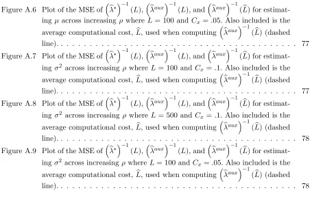
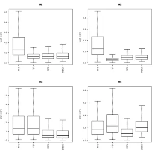
Design-based estimators

The MASE values and corresponding standard errors of the design-based estimators are dis-played in Table 2.2 for both SRS and Poisson sampling for n = 100 and σ = 0.1. Boxplots showing the distribution of ASE values are displayed in Figures 2.2 and 2.3. The ratio estima-torQb_D_|_R, position estimatorQb_D_|_POS, and both direct quantile-based estimatorsQb∗

D|RandQb

∗

D|D

are not included in these results because they performed significantly worse than the other estimators.

In general, Qb_D_|_DEN performed best among design-based estimators. Under M1, it had the lowest (or tied for the lowest) ASE values. Under M2,Qb_D_|_DENperformed the best ifσ = 0.3 (higher variance) butQb_D_|_Dperformed best ifσ = 0.1. Under M3 and M4,Qb∗_D_|_DEN always had the lowest ASE values with the exception ofn= 100, σ= 0.1, and SRS scenario, whereQb_D_|_PS performed best.

Model-based estimators