Attentive Query Network.

(1)

ABSTRACT

GUPTA, ARSHITA. Attentive Query Network. (Under the direction of Dr. Tianfu Wu).

Scene understanding is an important problem in modern high-level computer vision.

Currently a lot of effort is being put in developing algorithms that will help in the

3D reconstruction of an entire scene. Various present solutions proposed require human annotation like masking thus increasing the dependency of these algorithms on humans.

Further, once this masking is applied, they focus only on one object in the entire scene.

We wish to not only create a 3D representation of the object but generate the entire

scene from any user defined viewpoint different than the previously observed viewpoints.

This work takes a deep dive into the novel idea of scene rendering using query networks

[6] and further adds onto it a spatial attention mechanism. Unlike the other techniques,

this method relies entirely on the self-sufficient learning of the machine and removes any

involvement from humans.

The original Generative Query Network (GQN), although quite appreciable, takes millions of iterations to converge as it works towards generating the entire scene at

every iteration step. Generally, the walls, ground and sky occupy most of the image, the

network spends most of its time refining their representation and hardly focuses on the

more important objects in the room. We, therefore, introduce an attention mechanism

that will help to direct the focus on the objects of interest and give less attention to the

monotonous walls, thus rendering a refined scene which converges faster than the original

method. This attention mechanism will learn to put more importance on the foreground

objects in the image by providing with more weight and simultaneously assigning less

(2)

(3)

Attentive Query Network

by Arshita Gupta

A thesis submitted to the Graduate Faculty of North Carolina State University

in partial fulfillment of the requirements for the Degree of

Master of Science

Electrical Engineering

Raleigh, North Carolina

2019

APPROVED BY:

Dr. Edgar Lobaton Dr. Xu Xu

Dr. Tianfu Wu

(4)

DEDICATION

(5)

BIOGRAPHY

Arshita Gupta is a M.S. student in the Department of Electrical and Computer

Engi-neering at North Carolina State University. She pursued her Masters Thesis under the

guidance of Dr. Tianfu Wu, where she conducted research on generative network for 3D

scene understanding and rendering. Prior to joining NCSU, Arshita graduated with a

(6)

ACKNOWLEDGEMENTS

I firstly extend my gratitude to my advisor, Dr. Tianfu Wu, who has played a major role

in this research. Due to his ideas and encouragement to think outside the box, I was able

to complete this work. I thank Dr. Wu for his time and knowledge that he has shared

with me. He allowed this paper to be my own work, but directed me in the right direction

whenever I needed any help.

I would like to thank my committee members Dr. Xu Xu and Dr. Edgar Lobaton for

their generous support and time in supervising my thesis. A special thanks to Dr. Edgar Lobaton with whom I spent many hours pondering over the specifics of my thesis work

as well as coming up with a robust pipeline to bring sanity to this work.

I am extremely grateful for the open-access research papers and software which has

al-lowed me to learn, study and experiment with algorithms present in this modern research

period.

Last but not the least, I would like to express my very profound gratitude to my

par-ents and my brother for providing me with love, support and continuous encouragement

throughout my years of study and research. This accomplishment would not have been

(7)

LIST OF FIGURES

Figure 2.1 ith scene . . . 5

Figure 2.2 Tower Representation Network . . . 6

Figure 2.3 Generative Network . . . 7

Figure 2.4 Iterative construction of a painting . . . 9

Figure 2.5 Inner structure of ConvLSTM . . . 10

Figure 2.6 Residual learning with Skip connection . . . 11

Figure 2.7 Complete structure of GQN . . . 12

Figure 2.8 GQN results after equal interval. . . 13

Figure 3.1 Visualization for attention. Top: Soft Attention, Bottom: Hard At-tention . . . 15

Figure 4.1 Attention Mechanism . . . 17

Figure 4.2 Attentive Query Network . . . 19

Figure 4.3 Attentive Query Network . . . 20

Figure 4.4 Images from scene 1 with 1 object in the scene: Figure (a) to (e). Images from scene 2 with 2 objects in the scene: Figure (f) to (j). Images from scene 3 with 3 objects in the scene: Figure (k) to (o) 21 Figure 5.1 Comparing results of GQN and AQN after approximately 2500 steps. 23 Figure 5.2 Plot of Test MSE Loss vs epochs for GQN and AQN . . . 24

Figure 5.3 Comparing results of GQN and AQN + Lα after approximately 2500 steps. . . 25

Figure 5.4 Plot of Test MSE Loss vs epochs for GQN and AQN +Lα . . . . 26

Figure 5.5 Comparing results of GQN and AQN + Lβ after approximately 2500 steps. . . 27

(10)

Chapter 1 INTRODUCTION

1.1 Motivation

In 2018, DeepMind introduced Generative Query Network (GQN) [6], a framework to

represent scenes using only the extrinsic parameters of a camera and thus removing

any reliance on human defined labels, annotations or masking. The main idea of GQN is to take images from different viewpoints as inputs, construct a representation that

best describes the scene using all the images, and predict the image of the scene from a

different viewpoint which has not been observed earlier. The representation of the scene

is generated using a convolutional network while the core of this architecture consists

of an encoder and decoder pair of convolutional LSTMs. Without any prior domain

knowledge, the model is not only able to represent the object in the scene from any

unobserved viewpoint, but is able to reconstruct an accurate representation of the entire

scene from that unobserved view. It also learns about the texture and color of the wall,

ground, sky and additionally also includes the shadow due to any light source which may be present in the scene.

Although GQN is one of the best techniques available for reconstruction/generation

today, the downside of using GQN is that the network takes millions of step to generate

the perfect image. The simple argument here is that GQN takes a single sweep at the

entire image from all the viewpoints and tries to work on refining the entire output.

In a normal scene, many of the pixels in the image captures the three most frequently

occurring elements that is, the wall, ground and sky. Only a few pixels capture the objects

present in the scene. Due to this, the network spends most of its time refining the texture

(11)

on bringing clarity in the object like structures present in the scene. Thus, the main

challenge for such sequential models is learning exactly where to look at a given time in order to get an adequate representation of the entire scene.

Therefore, we introduce here an additional attention module that typically selects

where to read at any instance. The reading mechanism works by considering 2D Gaussian

filters which is inspired by DRAW (A Recurrent Neural Network For Image Generation)

[8].This mechanism, when applied to the original image, fits a grid of Gaussian filter over

the entire image thus giving more weight to the important areas and less weight to the

irrelevant regions. At every time step, it attends to the image and focuses on the most

important feature that will help in refining the generated image to as close to the original

image as possible. This task is challenging as images from all viewpoints have to be given attention at different locations. With this extra attention, we observe that the original

network is able to capture object like structure present in the scene alongside the wall,

ground and sky. Though not perfect, but a better representation of the scene can be

observed much faster than the original GQN.

1.2 Structure

The rest of the thesis work goes as follows: Chapter 2 first covers the general related work that has been done in 3D reconstruction. Next, we dive deep into the work that

this thesis is heavily based on which is Deepmind’s Generative Query Network (GQN)

[6]. We discuss, in detail, the architecture of GQN, followed by its working. We then raise

our concern on why this technique is slow and takes time to converge.

In our 3rd chapter, we talk about an attention mechanism that can help us assist

a more efficient GQN. We go in detail with the different kind of attention techniques

available and which one will assist us the best.

In Chapter 4, we talk about our new methodology which uses attention to give weight

to important features in our image. We explain in detail how we use this mechanism with the original GQN. Further, we talk about our experimental setup where we discuss our

data set and hardware details required.

We then take our reader to the result section in Chapter 5. We talk about the

promis-ing nature of our new method and additionally introduce another technique that can

assist in a better training of the original GQN.

(12)

Chapter 2 BACKGROUND

2.1 Related Work

GQN outperforms many algorithms that have been previously implemented for a similar

purpose. Traditional object reconstruction methods [27], [24] requires human annotators

to specify a mask around the object that has to be reconstructed. They also provide with a very generalized gray scale 3D reconstruction. GQN learns a more realistic reconstruction

of the entire scene including the color of object, texture and color of the walls and ground.

Many techniques focusing on 3D reconstruction rely on depth sensors or stereo

cam-eras for reconstruction of images [10]. GQN does not require any additional hardware

other than the camera that moves through the scene collecting images.

A few of these techniques require extra information from the image such as the

van-ishing line of a reference plane or vanvan-ishing point in a direction other than the one parallel

to the plane [4]. Similar methods [17], [9] put restrictions on the reconstructed objects

by placing various kinds of bounds on it. GQN, on the other hand, does not require any scene understanding before hand.

General reconstruction algorithms [12], [7] focus more on the generation of observed

images and currently does not hold any straightforward technique for generation of images

from unobserved views. The simple reason is that the features extracted in the first stage

of these techniques are not sufficient to give a wholesome understanding of the entire

scene.

Currently several researchers are seen putting efforts in cross view Image synthesis.

In some of the recent ones, Conditional GANs [19] was being used to generate street view

(13)

semantic layout of ground images. Several others have tried relating the problem between

the relation of aerial and ground images in [23], [13]. However these methods are highly specific as they generate images only from one particular direction.

There has been some work done in multi view synthesis from single objects [22]. Most

of the techniques that use CNN to generate [5], [28] generate image at once indicating

that all the pixels are conditioned on a single latent space. GQN on the other hand uses

Convolutional LSTM. This helps in generating images at every time step thus refining

the image on from the previously generated image.

2.2 Intoduction to GQN

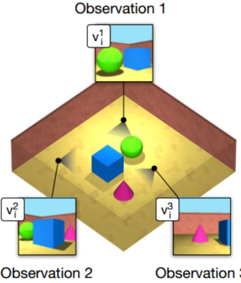
The concept of Generative Query Networks (GQN) was released by DeepMind in 2018

[6]. The idea behind this technique is that any 3D scene i can be represented by K 2D

images, denoted by xk

i, which are taken from K different viewpoints, denoted by vki.

GQN takes these xk

i images and vki viewpoints as inputs and, as an intermediate step,

constructs a representation r that best describes all the images and viewpoints for that

scene. After simple element-wise aggregation of these representations is done, GQN uses

this aggregated representation to predict an 2D image xq of the scene from a different

query viewpoint v_iq that has not been previously observed. Generally, it is not easy to generate image from an unobserved viewpoint as objects obstruct other objects and

even block some parts of themselves. GQN handles this problem by training stochastic

generators using conditional generative models. The prior knowledge that is learnt while

training leads to credible images being sampled out while testing.

As mentioned earlier, the input training dataset comprises a combination of the

view-points vk

i and their corresponding images xki from those viewpoints. This can be best

represented by D where:

D=(xki, vki) (2.1)

i∈ {1, ..., N} where N is the number of scenes in the data set.

k ∈ {1, ..., K} where K is the number of views for each scene.

vk

i is a viewpoint parametrized by a 5-dimensional vector (w, y, p) where w is the

three-dimensional position of the camera, yis the yaw and pis the pitch. The viewpoint

can be given by

ˆ

(14)

Figure 2.1: ith scene

xk_i is an RGB image captured from v_ik

2.3 Architecture of GQN

The entire Generative Query Network can be broken into 3 major parts. Each part has

been explained in detail below:

2.3.1 Representation Network

DeepMind has given three possible choices for the architecture of representation network

for GQN. We look closely at the tower representation architecture, given in Fig. 2.2, as

they claimed to have found this architecture to learn the fastest across data sets. We will also be working with this architecture for this entire thesis work.

(15)

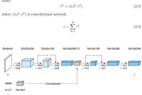
equa-tions:

rk =ψ(xk,ˆvk) (2.3)

where ψ(xk_,_v_ˆk_{) is convolutional network.}

r=

M

X

k=1

rk (2.4)

Figure 2.2: Tower Representation Network

For every image corresponding to each viewpoint in the scene, a representation r is

generated. As you can see from the Tower architecture shown in Fig. 2.2, the summary

of corresponding viewpoint to the image is concatenated in the middle of the

representa-tion network. All the representarepresenta-tions for a given scene, obtained from the Representarepresenta-tion

architecture, are element wise added to one another represented by R. Though the

tech-nique might seem very simple, it works great due to the fact that all the networks are

jointly trained.

Another technique that could have been used here,instead of element wise addition, is to concatenate all the representations rk _{. However, this representation would the be}

(16)

Figure 2.3: Generative Network

2.3.2 Generative Network

The Generative network uses a Convolutional LSTM, detailed explanation of

Convo-lutional LSTM is given in section 2.5, to generate images in a sequential manner.The

intuition behind using LSTM instead of Convolutional Neural network can be read from section 2.7. Coming back to the GQN model, there is an additional Skip connection [3]

added in the ConvLSTM, detailed explanation given in section 2.6, to assist

uninter-rupted gradient flow. This network, architecture given by Fig. 2.3, performs the bulk of

(17)

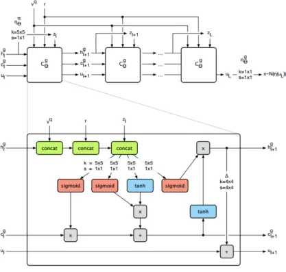
Prior factor:

πθl(·|v

q

, r, z<l) = N(·|ηθπ(h g

l)) (2.5)

where the latent variablez is split intoL latent variables and the convolutional network

ηπ θ(h

g

l) map the respective images to a Gaussian density.

Prior Sample:

zl ∼πθl(·|v

q_{, r, z}

<l) (2.6)

Convolutional LSTM state update:

(cg_l+1, hg_l+1) = ConvLST M_θg(vq, r, cg_l, hg_l, zl) (2.7)

wherevq _and _r _{corresponds to query viewpoint and the combined representation}

respec-tively, cg_l and hg_l are standard LSTM state variables.

Skip connection state update:

ul+1 =ul+ ∆(hgl+1) (2.8)

Observation sample:

x∼ N(xq|µ=η_θg(uL), σ =σt) (2.9)

where η_θg(uL) maps the inputs to the mean of Gaussian density.

Posterior Sample:

zl ∼qφl(·|x

q_{, v}q_{, r, z}

<l) (2.10)

2.3.3 Inference Network

The Inference network comprising of a standard Convolutional LSTM, shown below, is

dedicated entirely to the inference process.

(ce_l+1, he_l+1) = ConvLST M_φe(xq, vq, r, ce_l, he_l, hg_l, ul) (2.11)

where xq _{is the query image that we are trying to predict. The other equations used in}

original GQN paper are reiterated below:

Posterior factor:

qφl(·|x

q_{, v}q_{, r, z}

<l) =N(·|ηφq(h e

l)) (2.12)

(18)

Posterior sample:

zl ∼qφl(·|x

q

, vq, r, z<l) (2.13)

The Generator state update can now be written as:

(cg_l+1, hg_l+1, ul+1) = C_θg(vq, r, cg_l, hg_l, ulzl) (2.14)

2.4 Use of LSTM over CNN for generation

Many image generation approaches available today like in [18], generate the entire image

at once. This thus implies that all the pixels of the generated image will be conditioned

on one latent distribution. Basically, in most of these generation methods, the network

consists of a number of deconvolution layers stacked together. These map one single latent

distribution to bigger matrix at every deconvolution step and finally to an image.

Use of an LSTM network, like the ones used in [8] and [1], thus differs from the ’one shot’ generation networks in the sense that it constructs parts on the image and thus

the image is refined at every step. At every step the model improves upon its previously

generated image. Such a network thus follows a more natural form of image generation

similar to a real scenario where a person is drawing or painting a scene. The painter

starts with rough outlines of the scene and then gradually replaces it with precise lines

and shapes similar to the steps shown in Fig. 2.4

(19)

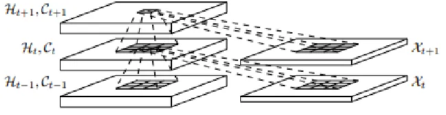
2.5 Convolutional LSTM

As mentioned in Generative Network in section 2.3, GQN uses a Convolutional LSTM

[21] to generate the query image xq_{. A convolutional LSTM is suitable for this task as}

we are dealing with generation of images. It combines the advantages of both LSTM and

convolutional networks. The LSTM method helps to iteratively construct images through

an accumulation of modifications produced by the decoder at every step, each of which

is observed by the encoder. The convolutional method, on the other hand, preserves the

local correlational structure present within the images.

Figure 2.5: Inner structure of ConvLSTM

The key equations of Convolutional LSTM have been mentioned below:

it =σ(Wxi ∗Xt+Whi∗Ht−1+Wci∗Ct−1+bi) (2.15)

ft=σ(Wxf ∗Xt+Whf ∗Ht−1+Wcf ∗Ct−1+bf) (2.16)

Ct =ft◦Ct−1+it◦tanh(Wxc∗Xt+Whc∗Ht−1+bc) (2.17)

ot=σ(Wxo∗Xt+Whi∗Ht−1+Wco∗Ct+bo) (2.18)

Ht=ot◦tanh(Ct) (2.19)

The most noticeable difference between this network and the usual LSTM is that all

(20)

ot of the ConvLSTM are 3D tensors whose last two dimensions are spatial dimensions.

2.6 Skip Connections

Figure 2.6: Residual learning with Skip connection

The most notable work using skip connection was done in Residual Neural Network

[11]. Shown in Fig. 2.6 the skip connection is represented by the curved arrow. This arrow

adds the input x to the output F(x). Now, the overall output of this entire section is

F(x) +x. Addition of this skip connection allows for uninterrupted flow between any layers. Many other techniques like [20] and [14] utilize such skip connections to allow for

later layers to learn simple features that were captured in the initial layers.

The motivation to use skip connections in the convolutional LSTM is to avoid any

problem that might arise due to vanishing gradients. This simple technique neither adds extra parameters nor increases any kind of complexity. It works by using activations from

the previous layer until the weights of next layer have been learnt. This, thus, speeds up

learning during training by reducing the influence of vanishing gradients as there are

less layers to propagate through. As the network approaches the end of the training, it

(21)

2.7 Working of GQN

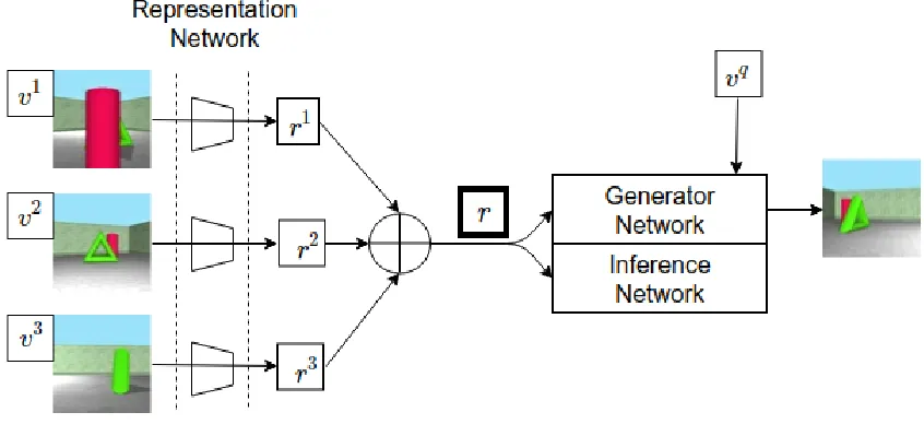
The basic working of GQN can be understood from Fig. 2.7.

Figure 2.7: Complete structure of GQN

At each gradient step, a batch of B scenes with M observations is sampled out. A

representationrk is formed from the images and their corresponding viewpoints through

the representation network by using the Eq. 2.3. All the representations are aggregated

together to form one single representation r that best defines the entire 3D scene given by Eq. 2.7. The generative network uses this representation of the 3D scene to generate

an image from an unobserved viewpoint using equations in section 2.3.2 and 2.3.3.

GQN uses a standard variational approximations consisting of two main terms, that

is, the reconstruction likelihood and a regularization term and uses adaptive gradient

descent for optimisation.

F(θ, φ) =_E(x,v)∼D,z∼qφ "

−lnN(xq|η_θg(uL)) + L

X

l=1

KL

h

N(·|η_φq(he_l)||N(·|ηπ_θ(hg_l) i

#

(2.20)

(22)

2.8 Drawbacks of GQN

Although GQN allows for a clean representation of images from unobserved viewpoints,

it needs millions of steps to converge. If we observe the images collected from the different

viewpoints, we can undoubtedly conclude that the ratio of pixels describing the three basic

elements that is the sky, walls and ground is higher than the pixels that represent the

object of interest in these images. Although GQN works well for such simulated scenes, it

can fail dramatically in real life scenarios where the ratio, mentioned above, is very high.

The reason for this behaviour is the simple fact that GQN reads the entire image from

all the viewpoints in one single swipe and forms a representation of it. It now tries to generate an output and tries to rectify this output based on the representation collected

at the first step. Because the network forms a representation of the entire image, the

aggregated representation finally formed consists high information from the three basic

elements with little knowledge of the objects present.

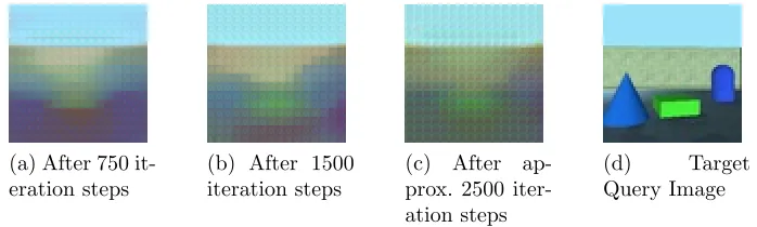
(a) After 750 it-eration steps

(b) After 1500 iteration steps

(c) After ap-prox. 2500 iter-ation steps

(d) Target Query Image

Figure 2.8: GQN results after equal interval.

We implemented GQN with the exact same specification provided in [6] and found

the results given in Fig. 2.8 which shows the generated query image for a test sample.

All the images above in Fig. 2.8a, 2.8b, 2.8c have each been generated at an interval of

750 iteration steps. As you can observe from this figure, the images Fig. 2.8b and 2.8c

generated show very little improvement from their previous image. There is also a lot of blurring in these images.

Looking at these results, we therefore feel the need of an additional attention module

that can help to focus on the important objects present in the foreground in every image,

thus forming a more meaningful representation of these objects of interest in the original

(23)

Chapter 3 ATTENTION MECHANISM

Attention is required in order to focus onto particular objects which hold more importance

than the rest of the scene. This helps us to filter out irrelevant or highly repetitive features

from scene thus assisting us to bring out supreme image features from localized areas.

Lately attention mechanisms are being applied in many deep learning problems especially

computer vision. [25].Many other [2] and [15] have explored the other forms of attention

mechansim. Let’s look at two major types of attention.

3.1 Types of attention

3.1.1 Hard Attention Mechanism: Stochastic Learning

This mechanism selects a patch of image to attend at each particular instance. The

mech-anism does a hard assignment where images that are considered not important are given

a value of 0 while the rest retain their pixel values. The parameters of Hard attention

mechanism are learnt and can be represented by a multinoulli distribution. The location

where the model decides to focus needs to be sampled out from this multinoulli

distribu-tion. For hard attention mechanism in images, this location is given by the bounding box. Every pixel outside the box is made 0 while all the pixels inside the box retain their

val-ues. Now, because of the sampling technique used here, the gradient has to be computed

to Monte Carlo and is subject to high variance. Therefore, many tricks are required to

train such hard attention mechanisms and there is very little regularity across

implemen-tations. Recently work has been in the implementing of Hard Attention Learning Visual

(24)

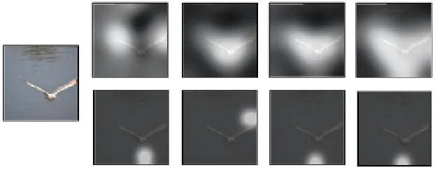
Figure 3.1: Visualization for attention. Top: Soft Attention, Bottom: Hard Attention

3.1.2 Soft Attention Mechanism: Deterministic Learning

Learning stochastic attention ( Hard attention mechanism) requires sampling the

atten-tion locaatten-tion at each time, instead we can formulate a deterministic attenatten-tion model. This deterministic model can be computed using a soft attention weighted annotation

vector. This entire mechanism is deterministic and therefore an end-to end training is

possible using standard back propagation. In short, Soft attention method allows for a

weighted mask over the image. What this means is that, soft attentions computes weight

wij for every pixelxij in imagex. This weight tells us how relevant a cell is. By applying

these set of weights over the image, this mechanism gives less credit to irrelevant regions

(25)

Chapter 4 METHODOLOGY

In our second chapter, we mentioned the challenge that we could face while training our

Generative Query Network proposed in [6]. In this chapter we introduce our attention

techniques to tackle the problems mentioned earlier.

Firstly, we introduce our Attentive Query Network, which uses an attention

mecha-nism to restrict the representation networks input to only a limited region from every

image in that scene. Thus at every step, the network decides what to read. It achieves this

task by applying grid of 2D Gaussian filters, similar to the attention mechanism used in DRAW [8], on every image from the scene. At every step, the attention mechanism uses

the hidden state, of the generator network, to learn the parameters needed to highlight

important regions from an image. Combined with the corresponding viewpoint of the

image, it is able to learn parameters that assists it to attend the required area for the

given viewpoint. Thus at every step, the representation network focuses on a particular

region of the image.

4.1 Working of AQN

The basic working of Attentive Query Networks can be understood from Fig. 4.1. At

every time step, attention is given to the input images xk

i individually. h g

l from the

previous time step is concatenated with the corresponding vk

i for a given image xki. This

concatenated vector is then used to learn the grid parameters (gx, gy,logσ2,logγ). Our

method differs from the original DRAW [8] in the fact that we are using both hg_l and

v_ik for attention. Additionally, unlike in DRAW, where a patch of image is extracted,

(26)

gaussian filters (Fx, Fy, γ), obtained from grid parameters, over the entire image. This

filter puts large weight on important objects and less weight on the redundant regions. We do not extract patches like in the original DRAW paper as we fear that

extract-ing small patches and zoomextract-ing in will cause blurrextract-ing in the generated image. As the

original GQN already faces the issue of blurring, we think its better to work with the

entire image than just a patch. Also, we do face situations where we have 2-3 objects at

different locations in the scene. Extracting patches from the image will lead to complete

ignorance of other objects in the image. Instead of completely removing a second object,

while attending the first object, we give this second object some little weight that will

help to further strengthen the spatial relationship between all the objects in the scene.

Additionally, this ensures that the input to the representation model is of constant shape, which indirectly will result in a better learning of the representation layer.

We want our readers to note two things: 1. Firstly, we are currently assuming that

we are only working with one scene and therefore the subscript i has been removed for

simplicity. 2. Secondly, although we have mentioned that we are using grid of gaussian

filters, we have shown just one 2D gaussian filter in the figure 4.1 and 4.2 for simplicity.

Let’s take a closer look into the ’attention’ mechanism of our network:

Given an input image xk, all four attention parameters are dynamically determined

at each time step via a linear transformation L of the generator hidden output hg con-catenated with the corresponding viewpointvk _{given in fig. 4.1}

(27)

[gx, gy,logσ2,logγ] =L[hgkvk] (4.1)

where gx and gy are the grid centres. σ2 is the isotropic variance of the Gaussian filters

and γ that multiplies the filter response.

Once we have the grid centres, we can use it to find the mean of gaussian filter for

every pixel in the image using the equations mentioned below.

µi_X =gX + (i−A/2−0.5) (4.2)

µi_Y =gY + (i−B/2−0.5) (4.3)

where A and B is the shape of the xk.µi_X andµi_Y are the mean locations of the filter

at row i and column j.

Given the attention parameters, the horizontal and vertical filter matricesFX and FY

can be defined as:

FX[i, a] =

1

ZX

exp −(a−µ

i X)2

2σ2

!

(4.4)

FY[i, b] =

1

ZY

exp −(b−µ

i Y)2

2σ2

!

(4.5)

here a, b is a point in the input image. We finally get our context image:

xk_att=γ[FY, xk, FXT] (4.6)

We should note that the filter is applied to every channel in the input image xk

individ-ually. The final xk_att is obtained by concatenating these three channels in the end.

This is the the new input image that is sent through representation layer. The next steps followed are similar to GQN mentioned in Chapter 2, section 2.3.

We would like to stress on the fact that readmechanism in DRAW takes only the hg

of the previous time step. In contrast to this, we use a simple concatenation of both hg

and the corresponding viewpointvk _{for the image}_xk_{. If we omit this concatenation step,}

then we are basically giving same attention for all the different viewpoints. This could

mislead our network as objects of importance can be at different location for images

from different viewpoints. Hence, the read mechanism should apply attention at different

(28)

Figure 4.2: Attentive Query Network

we observe that the model performs well. Since, the representation, generation and

at-tention mechanism are trained jointly, gradients from the generative network encourage

the attention network to learn better parameters at every iteration step.

4.2 Loss Function

The original loss function used by GQN has been given by the Eq.2.20. However, we do

realise that the query network’s main goal is to be able to generate an image as realistic

as possible. To make the our modified AQN model more robust we propose two methods

that modify the original loss function in Eq. 2.20

• LossLα:

This new loss can be represented by the following equations mentioned below:

Loss = reconstruction loss + regularization term + Lα

where

Lα = L

X

(29)

Figure 4.3: Attentive Query Network

This additionally mean square error term is calculated sequentially using images generated at every time step with the target image. We believe that this added extra

term will help the network pay more attention on how accurate the generation of

the network really is.

• LossLβ:

This new loss can be represented by the following equations mentioned below:

Loss = reconstruction loss + regularization term + Lβ

where

Lβ = L

X

l=1

(l

L ×M SELoss(ˆxql, xql)) (4.8)

This term, like the previous one, is also calculated sequentially at every time step.

For this particular loss function, we give less weight to the initially generated image

and give more weight to he last image generated in the sequence.

4.3 Experimental Setup

4.3.1 Data set

DeepMind has provided with seven different types of data set containing different kinds

(30)

specifically used the ’rooms ring camera’ data set. This data set consists of several scenes

of random objects placed in a square room of size 7x7 units. The scenes differ from one another with respect to the different wall textures (in all 5 different colors possible), floor

color (in all 3 colors possible) and even the shape of objects (7 shapes possible) and their

different colors that they contain. Another point to keep in mind is that the camera,

that is used to capture the images, only moves on a fixed ring and always faces the room

center. The rooms had a maximum of 3 objects per scene but less are also possible. An

example of scenes containing 1, 2 and 3 objects has been shown in Fig 4.4

(a) Image 1 (b) Image 2 (c) Image 3 (d) Image 4 (e) Image 5

(f) Image 1 (g) Image 2 (h) Image 3 (i) Image 4 (j) Image 5

(k) Image 1 (l) Image 2 (m) Image 3 (n) Image 4 (o) Image 5

Figure 4.4: Images from scene 1 with 1 object in the scene: Figure (a) to (e). Images from scene 2 with 2 objects in the scene: Figure (f) to (j). Images from scene 3 with 3 objects in the scene: Figure (k) to (o)

4.3.2 Hyper-parameter setup for training

We trained all our model using 8 images per scene. Due to our hardware limitations, we

were unable to go beyond a batch size of 4. The sequence length of our ConvLSTM was 5.

(31)

from the images and viewpoints. We have trained both the GQN and AQN model under

same specifications for about 2500 steps.

4.3.3 Optimizer and Scheduler

We use an Adam optimizer where the learning rate used by the Adam algorithm, varies

with the training step s and is given by the Eq:4.9

γs=µs

p1−βs

2

1−βs 1

(4.9)

where β1 = 0.9,β2 = 0.999 and µs is the learning rate at training step s with annealing

and is given by the Eq. 4.10

µs =max

µf + (µi−µf)(1−

s n), µf

(4.10)

where µi = 5×10−4 , µf = 5×10−5 and η = 1.6×106

4.3.4 Hardware Details

The original GQN has been trained on 4 NVidia K80 GPUs. We have trained our model

(32)

Chapter 5 RESULTS

We now assess the ability of Attentive Query Network to generate images from unobserved

view points and compared it with the original Generative Query Network. We have shown

three sets of results here. For quantitative analysis, we use Mean Square Error (MSE)

Loss on our generated Test data set.

5.1 Experiment 1

(a) Scene 1 us-ing GQN

(b) Scene 1 us-ing AQN

(c) Scene 1 Tar-get Query Im-age

(d) Scene 2 us-ing GQN

(e) Scene 2 us-ing AQN

(f) Scene 2 Tar-get Query Im-age

(33)

In our first experiment, we have shown the generated query image from our Test data

set using both Generative Query Network Fig. 5.1a and Fig. 5.1d and Attentive Query Network Fig. 5.1b and Fig. 5.1e, generated after approximately 2500 iteration steps, and

compared with the target query image Fig. 5.1c and Fig. 5.1f.

We show two examples here. In scene 1, We can observe from the given Fig. 5.1a,

while the Generative Query Network is able to get the exact color of the walls, sky and

ground, the objects generated in the foreground are very blurred. The three objects,

shown in Fig. 5.1c, seem to have been completely merged into one another as shown in

Fig. 5.1a. On the other hand, Attentive Query Network shows to have generated a better

image, Fig. 5.1b with more clear object as compared to GQN.

In scene 2,we observe that, although GQN is able to detect the blue object in the right, Fig. 5.1d, the generated image seems to have spread the blue object throughout

the image. On the other hand, AQN , Fig, 5.1e has been able to create the object in its

restricted area. The images generated by AQN resembles the target query image Fig. 5.1f

more than the images generated by GQN for both scene 1 and 2.

Figure 5.2: Plot of Test MSE Loss vs epochs for GQN and AQN

Fig. 5.2 shows the change in MSE Loss for test data set with respect to the epochs.

(34)

both GQN (blue) and AQN (red), we observe that although AQN starts with a higher

loss, there is a larger slope associated with it. AQN gradually starts performing better than the original GQN.

5.2 Experiment 2

We did a second experiment where we added an additional loss Lα to the original GQN

loss, also explained in section 4.2.

After running this experiment for scene 1 we were able to observe a green rectangle,

Fig. 5.3b at the center, similar to the target image Fig. 5.3c. For our second scene, we observe a more concentrated blue object in the generated image, Fig. 5.3e.

Similar to our first experiment, we plot a linear trend line for both GQN (blue) and

AQN + Lα (pink) shown in Fig. 5.4, and once again observe that AQN + Lα, although

starts with a higher loss, gradually starts performing better than the original GQN. There

is a larger slope associated with this new technique. We can confidently say that AQN

+ Lα was able to outperform both GQN and AQN.

(b) Scene 1 us-ing AQN +Lα

(e) Scene 2 us-ing AQN +Lα

(35)

Figure 5.4: Plot of Test MSE Loss vs epochs for GQN and AQN + Lα

5.3 Experiment 3

In our third experiment, we modified our extra loss Lα to Lβ, explained in section

ex-plained in section 4.2. This experiment did not yield expected results, however we still

felt the need to show our results as an ablation study so as to help the readers understand

how the generative model gets affected with change in loss function.

From Fig. 5.5b, we can we can observe that there is more blurring than the image

generated by original GQN method shown in Fig 5.5a.This could possibly suggest that every image that is being generated in the LSTM sequence is important and a weighted

mean square error loss might imbalance this distribution. The brighter tinge at the center

of the Fig. 5.5b adds on to the possibility that giving higher value to the image being

generated at the end of the sequence, can give unnecessary weight to thoepixels and thus

cause the distortion in the image generated. We see a similar problem in Fig. 5.5e that

was generated for scene 2.

Additionally, we plot a similar linear trend line for both GQN (blue) and AQN + Lβ

(yellow) shown in Fig. 5.6. On Observing this plot, this extra weight Lβ does not seem

(36)

(b) Scene 1 us-ing AQN

(e) Scene 2 us-ing AQN +Lβ

Figure 5.5: Comparing results of GQN and AQN + Lβ after approximately 2500 steps.

(37)

Chapter 6 CONCLUSIONS

6.1 Summary

This thesis talks about a new method Generative Query Networks, introduced by

Deep-Mind [6] in 2018. We demonstrate its ability to generate an image of a scene from an

unobserved viewpoint. We argue the fact that original GQN takes time to converge and thus and add an attention mechanism on top of it. This soft attention mechanism using

gaussian filters help to give more importance to the relevant features and less weight

to the irrelevant and repetitive features. We further add an extra Loss term to its loss

function in order to assist better generation of this Query Network. Our method, when

trained for the same duration as the GQN seems to slightly improve the network and

give better generated results. With such promising results, we strongly believe that with

improved hardware, we can generate highly realistic and natural like results.

6.2 Future Work

For this thesis work, we have limited ourselves to the fact every image is linked to its

corresponding viewpoint. However, we have not looked into the possibility that there

could exist a relation between the different viewpoints that exist in the data set. Building

on this, we could formulate a weighted relation of the different viewpoints with the

query viewpoint. Weights would be assigned to images in the order of how close the

corresponding viewpoints are to the query viewpoint, giving higher weight to the image

(38)

weighted average function in GQN. We provide a little example to give our readers a

little glimpse of this new function. In general, we replace the original function mentioned in Eq. 2.7 by a new weighted averaging function given in Eq. 6.1

(a) Original aggregation function (b) Modified aggregation function

r =

M

X

k=1

(wk×rk) (6.1)

where wk _{could be given by a simple equation given 6.2}

wk = α

d(vq_{, v}k₎ (6.2)

(39)

REFERENCES

[1] Jimmy Ba, Volodymyr Mnih, and Koray Kavukcuoglu. Multiple object recognition with visual attention. arXiv preprint arXiv:1412.7755, 2014.

[2] Denny Britz, Anna Goldie, Minh-Thang Luong, and Quoc Le. Massive exploration of neural machine translation architectures. arXiv preprint arXiv:1703.03906, 2017.

[3] V´ıctor Campos, Brendan Jou, Xavier Gir´o-i Nieto, Jordi Torres, and Shih-Fu Chang. Skip rnn: Learning to skip state updates in recurrent neural networks.arXiv preprint arXiv:1708.06834, 2017.

[4] Antonio Criminisi, Ian Reid, and Andrew Zisserman. Single view metrology. Inter-national Journal of Computer Vision, 40(2):123–148, 2000.

[5] Alexey Dosovitskiy, Jost Tobias Springenberg, Maxim Tatarchenko, and Thomas Brox. Learning to generate chairs, tables and cars with convolutional networks.IEEE transactions on pattern analysis and machine intelligence, 39(4):692–705, 2017.

[6] SM Ali Eslami, Danilo Jimenez Rezende, Frederic Besse, Fabio Viola, Ari S Morcos, Marta Garnelo, Avraham Ruderman, Andrei A Rusu, Ivo Danihelka, Karol Gregor, et al. Neural scene representation and rendering. Science, 360(6394):1204–1210, 2018.

[7] Ian Goodfellow, Jean Pouget-Abadie, Mehdi Mirza, Bing Xu, David Warde-Farley, Sherjil Ozair, Aaron Courville, and Yoshua Bengio. Generative adversarial nets. In Z. Ghahramani, M. Welling, C. Cortes, N. D. Lawrence, and K. Q. Weinberger, editors, Advances in Neural Information Processing Systems 27, pages 2672–2680. Curran Associates, Inc., 2014.

[8] Karol Gregor, Ivo Danihelka, Alex Graves, Danilo Jimenez Rezende, and Daan Wierstra. Draw: A recurrent neural network for image generation. arXiv preprint arXiv:1502.04623, 2015.

[9] Feng Han and Song-Chun Zhu. Bayesian reconstruction of 3d shapes and scenes from a single image. In First IEEE International Workshop on Higher-Level Knowledge in 3D Modeling and Motion Analysis, 2003. HLK 2003., pages 12–20. IEEE, 2003.

[10] Tal Hassner and Ronen Basri. Example based 3d reconstruction from single 2d images. In2006 Conference on Computer Vision and Pattern Recognition Workshop (CVPRW’06), pages 15–15. IEEE, 2006.

(40)

[12] Diederik P Kingma and Max Welling. Auto-encoding variational bayes. arXiv preprint arXiv:1312.6114, 2013.

[13] Tsung-Yi Lin, Serge Belongie, and James Hays. Cross-view image geolocalization. In Proceedings of the IEEE Conference on Computer Vision and Pattern Recognition, pages 891–898, 2013.

[14] Jonathan Long, Evan Shelhamer, and Trevor Darrell. Fully convolutional networks for semantic segmentation. In Proceedings of the IEEE conference on computer vision and pattern recognition, pages 3431–3440, 2015.

[15] Minh-Thang Luong, Hieu Pham, and Christopher D Manning. Effective approaches to attention-based neural machine translation. arXiv preprint arXiv:1508.04025, 2015.

[16] Mateusz Malinowski, Carl Doersch, Adam Santoro, and Peter Battaglia. Learning visual question answering by bootstrapping hard attention. In Proceedings of the European Conference on Computer Vision (ECCV), pages 3–20, 2018.

[17] Emmanuel Prados and Olivier Faugeras. Shape from shading. In Handbook of mathematical models in computer vision, pages 375–388. Springer, 2006.

[18] Alec Radford, Luke Metz, and Soumith Chintala. Unsupervised representation learning with deep convolutional generative adversarial networks. arXiv preprint arXiv:1511.06434, 2015.

[19] Krishna Regmi and Ali Borji. Cross-view image synthesis using conditional gans. In Proceedings of the IEEE Conference on Computer Vision and Pattern Recognition, pages 3501–3510, 2018.

[20] Olaf Ronneberger, Philipp Fischer, and Thomas Brox. U-net: Convolutional net-works for biomedical image segmentation. In International Conference on Medical image computing and computer-assisted intervention, pages 234–241. Springer, 2015.

[21] Xingjian SHI, Zhourong Chen, Hao Wang, Dit-Yan Yeung, and Wai-kin Wong. W.-c. woo. convolutional lstm network: A machine learning approach for precipitation nowcasting. Advances in Neural Information Processing Systems, 28:802–810, 2015.

[22] Maxim Tatarchenko, Alexey Dosovitskiy, and Thomas Brox. Multi-view 3d mod-els from single images with a convolutional network. In European Conference on Computer Vision, pages 322–337. Springer, 2016.

(41)

[24] Jiajun Wu, Chengkai Zhang, Xiuming Zhang, Zhoutong Zhang, William T Freeman, and Joshua B Tenenbaum. Learning 3D Shape Priors for Shape Completion and Reconstruction. In European Conference on Computer Vision (ECCV), 2018.

[25] Kelvin Xu, Jimmy Ba, Ryan Kiros, Kyunghyun Cho, Aaron Courville, Ruslan Salakhudinov, Rich Zemel, and Yoshua Bengio. Show, attend and tell: Neural image caption generation with visual attention. In International conference on machine learning, pages 2048–2057, 2015.

[26] Menghua Zhai, Zachary Bessinger, Scott Workman, and Nathan Jacobs. Predicting ground-level scene layout from aerial imagery. InProceedings of the IEEE Conference on Computer Vision and Pattern Recognition, pages 867–875, 2017.

[27] Xiuming Zhang, Zhoutong Zhang, Chengkai Zhang, Joshua B Tenenbaum, William T Freeman, and Jiajun Wu. Learning to Reconstruct Shapes from Un-seen Classes. In Advances in Neural Information Processing Systems (NeurIPS), 2018.

Attentive Query Network.

ABSTRACT

DEDICATION

BIOGRAPHY

ACKNOWLEDGEMENTS

TABLE OF CONTENTS

LIST OF FIGURES

Chapter 1

INTRODUCTION

1.1

Motivation

1.2

Structure

Chapter 2

BACKGROUND

2.1

Related Work

2.2

Intoduction to GQN

2.3

Architecture of GQN

2.3.1

Representation Network

2.3.2

Generative Network

2.3.3

Inference Network

2.4

Use of LSTM over CNN for generation

2.5

Convolutional LSTM

2.6

Skip Connections

2.7

Working of GQN

2.8

Drawbacks of GQN

Chapter 3

ATTENTION MECHANISM

3.1

Types of attention

3.1.1

Hard Attention Mechanism: Stochastic Learning

3.1.2

Soft Attention Mechanism: Deterministic Learning

Chapter 4

METHODOLOGY

4.1

Working of AQN

4.2

Loss Function

4.3

Experimental Setup

4.3.1

Data set

4.3.2

Hyper-parameter setup for training

4.3.3

Optimizer and Scheduler

4.3.4

Hardware Details

Chapter 5

RESULTS

5.1

Experiment 1

5.2

Experiment 2

5.3

Experiment 3

Chapter 6

CONCLUSIONS

6.1

Summary

6.2

Future Work

REFERENCES