ABSTRACT
ARKATKAR, ISHA. ALACRI2TY: Lossless Data Compression for Analytics-driven Query Processing. (Under the direction of Nagiza F. Samatova.)
Analysis of scientific simulations is highly data-intensive and is becoming an increasingly
important challenge. Peta-scale data sets require us to look for alternative ways of performing query-driven analyses. This thesis is an attempt in the direction of query processing over
loss-lessly compressed scientific data. We propose ALACRI2TY (Analytics-driven Lossless dAta Compression for Rapid In-situ Indexing, sToring, and querYing), which at its core consists of two components: lossless compressor and query processing engine over compressed data.
ALACRI2TY’s compression component performs compression of double precision scientific data by unique value-based binning. Based on significant bit splitting,ALACRI2TY improves compression ratios over general-purpose compression utilities. It then indexes the metadata
about the compression rather than the data to enable light-weight index storage. The query
processing engine answers range queries over this compressed data with a low degree of unnec-essary decompression.
ALACRI2TY’s methodology involving compression and binning enables (1) Indexing with a total storage requirement (data+index) of less than 135% (versus 200-300% in existing sci-entific database systems); (2) Data access at multiple precision levels of detail necessitated by
the varying sensitivity of analytical kernels (e.g., low-precision for histograms and descriptive
statistics, medium-precision for clustering, and full-precision for Fourier analysis); (3) Robust performance across univariate as well as multi-variate query constraints via efficient
bitmap-based aggregation of partial results.
Altogether, these capabilities yield a multi-fold improvement in query response time over
state-of-the-art systems such as FastBit, MonetDB, and SciDB when tested on several
c
Copyright 2012 by Isha Arkatkar
ALACRI2TY: Lossless Data Compression for Analytics-driven Query Processing
by Isha Arkatkar
A thesis submitted to the Graduate Faculty of North Carolina State University
in partial fulfillment of the requirements for the Degree of
Master of Science
Computer Science
Raleigh, North Carolina
2012
APPROVED BY:
Rada Chirkova Kemafor Anyanwu
BIOGRAPHY
Isha Arkatkar earned her Bachelor’s of Technology in Computer Engineering form College of
Engineering, Pune, India in 2008. After graduating she worked for two years at Microsoft, India Development Center as a Software Development Engineer in Test. She enrolled as a
master’s student in Computer Science at North Carolina State University in Fall 2010. She
ACKNOWLEDGEMENTS
I would like to take this opportunity to thank all the people who directly or indirectly
con-tributed in completion of my thesis. First and foremost, I would like to thank my advisor, Dr. Nagiza Samatova, for her invaluable guidance throughout the course my graduate studies. This
thesis would not have been possible without her support, motivation and the expertise she has
shared to guide me through the thesis. I would also like to thank my committee members, Drs. Rada Chirkova and Kemafor Anwanyu, for reviewing my work and providing insightful
feedback.
I would also like to express gratitude to the other members of Dr. Samatova’s research group for their moral support, as well as for collaborating in the research work. I would especially
like to thank Sriram Lakshminarasimhan, John Jenkins, David Boyuka, Zhenhuan Gong, Eric
R. Schendel and Neil Shah for their contributions in the work presented here.
Lastly, I want to thank my father, sister and my fianc´e, for their unwavering support and
TABLE OF CONTENTS
List of Tables . . . vi
List of Figures . . . vii
Chapter 1 Introduction . . . 1
1.1 Reducing storage footprint of data by lossless compression . . . 2
1.2 Efficient range query processing with light-weight index . . . 3
1.3 Sensitivity of analytical kernels to precision levels . . . 4
Chapter 2 Compression Methodology . . . 6
2.0.1 Compression . . . 6
2.0.2 Choosing a Partition Size . . . 10
2.1 Lossless Compression Performance . . . 10
Chapter 3 Univariate Query Processing. . . 13
3.1 Index Generation . . . 13
3.2 Query Processing: File Layout . . . 15
3.2.1 Query Processing: Range Queries . . . 15
3.3 Results And Discussions . . . 16
3.3.1 Experimental Setup . . . 16
3.4 End-to-End Query Performance Evaluation . . . 17
3.4.1 Variable-Centric queries . . . 17
3.4.2 Region-Centric queries . . . 19
3.4.3 Needle in a Haystack Experiment . . . 19
3.4.4 Performance analysis . . . 20
Chapter 4 Multivariate Query Processing . . . 22
4.1 Challenges and Strategies . . . 22
4.2 Heterogeneous Query Process . . . 22
4.2.1 Overview . . . 22
4.2.2 Multi-variate Constraint Processing . . . 24
4.2.3 Spatial Index Bin Partitioner . . . 25
4.2.4 Cost Analysis . . . 28
4.2.5 Query Processing Evaluation . . . 33
Chapter 5 Precision-based Level of Detial . . . 37
5.1 Sensitivity of Analytical Kernels to PLoDs . . . 37
5.2 Precision-based Level of Detail . . . 38
5.2.1 Evaluation of Precision Level of Detail . . . 39
LIST OF TABLES
Table 2.1 Compression ratio for different data partition sizes. Original GTS
Poten-tial data is 3,414,682,240 bytes (2,561,011,680 low-order bytes). . . 10
Table 2.2 Compression metrics for various methods, against ALACRI2TY with a preference for compression (AC, using bzip2) and a preference for through-put (AT, using zlib). . . 11
Table 2.3 Compression Throughput for various methods, against ALACRI2TY with a preference for compression (AC, using bzip2) and a preference for throughput (AT, using zlib). . . 12
Table 2.4 Decompression Throughput for various methods, against ALACRI2TY with a preference for compression (AC, using bzip2) and a preference for throughput (AT, using zlib). . . 12
Table 3.1 Query index generation throughput and storage footprint . . . 16
Table 3.2 Response time (sec.) for the needle in a haystack experiment. ALACRI2TY used a 64 MB partition size. . . 20
Table 4.1 Parameters influencing query response time. . . 28
Table 4.2 Parameters for value retrieval estimation. . . 30
Table 4.3 Hardware and data parameters used in cost model. . . 32
Table 4.4 Cost model-based and actual response timings. . . 32
Table 5.1 Histogram error rates. . . 38
Table 5.2 Misclassification rates for k-means clustering. Sample size is 100,000 ran-dom 2-D points. . . 38
LIST OF FIGURES
Figure 2.1 Compression methodology, described in Section 2.0.1. The bitmap index is used for compression, while the spatial index is used in query processing. 7 Figure 2.2 Cumulative growth of the number of distinct higher order 2-byte and
3-byte patterns for increasing data size. The number of distinct byte patterns is plotted on a logarithmic scale. . . 8 Figure 2.3 Bin distribution for two scientific datasets. . . 9
Figure 3.1 Building a spatial index for query processing, compared to the compres-sion index. Row Id corresponds to a spatial index within a partition. . . . 14 Figure 3.2 Metadata file format. . . 15 Figure 3.3 Query processing methodology, taking into account metadata, index, and
compression data fetching and aggregating. . . 15 Figure 3.4 Comparison of speedup of ALACRI2TY overFastBit, and sequential
scans, for variable-centric queries when the query selectivity is varied from 0.001% to 10.0%. . . 18 Figure 3.5 Comparison of response return by FastBit against ALACRI2TY for
region-centric queries with varying number of query hits. . . 19 Figure 3.6 Comparison of Computation and I/O time distribution forALACRI2TY
for different query types over varying selectivity. On the other hand, FastBit spends over 90% of the time on I/O. . . 21
Figure 4.1 Overview of ALACRI2TYQuery Processing Engine, on a per-partition level. Input Q is a query of the form (SR, SV, VC, DC), where SR →
select region (X, Y), SV →list of variable values to retrieve (for example,
Select region, [V1]), VC → list of variable constraints (for example, (x < V2< y) AND (x1 < V3 < y1) ),DC →list of constraints on dimension. 23
Figure 4.2 High-level overview of the Bin Partitioner that divides the given sorted list of spatial indices into multiple lists of bins touched based on the alternate index, with an example. . . 26 Figure 4.3 Speedup compared to Query response time forALACRI2TY for range
queries with various selectivity and variable constraints (VC - number of
variable constraints, S - selectivity). . . 34 Figure 4.4 Speedup compared to Query response time forALACRI2TYfor queries
returning spatial region / value tuples, with various selectivity and vari-able constraints (VC - number of variable constraints, S - selectivity). . . 34
Figure 4.5 Query response time for queries returning spatial regions, with fixed selectivity with respect to spatial constraints and varying selectivity on variable constraints within sub-volume. . . 35 Figure 4.6 Query response time for queries returning regions and values with the
Figure 4.7 Query response time for queries returning only regions with the increas-ing number of variables. . . 36
Chapter 1
Introduction
Increasingly complex simulation models, used to simulate dynamics of various scientific pro-cesses, generate tera-bytes of data per run. The massive size of data generated from scientific
applications pose interesting challenges in managing and performing exploratory analysis of
data. On the one hand, the large data sizes necessitate lossless compression of data before writing to disk. On the other, compressing the data set in its entirety using general-purpose
compression utilities would hinder the data analytics procedure due to the prohibitive costs of
full dataset compression. Also, full context data analysis over the entire dataset is restrained by the limits of computer memory and I/O bandwidth. Thus, new paradigms are needed to
perform efficient analytics on extreme-scale data. It deems necessary to formulate a method for
reducing the storage footprint of data while at the same time maintaining the query processing capability. Thus, new paradigms are needed to perform efficient analytics over compressed
extreme-scale data without the need to decompress the entire dataset, based on regions of
interest to scientists.
Often times, scientists have some prior knowledge about the regions of interest in their data.
This makes aknowledge priors approach to data analytics a promising way to restrict data to smaller and more practical sizes. For example, fusion scientists aiming to understand plasma turbulence might formulate analyses questions involving correlations of turbulence intensities
in different radial zones (0.1< ψ <0.15; 0.3< ψ <0.35; 0.5< ψ <0.55; 0.7< ψ <0.75; 0.9< ψ < 0.95). Likewise, climate scientists aiming to understand factors contributing to natural disasters might limit their search to particular regions or perhaps only a single region.
Formulating queries on scientific simulation data constrained on variables of interest is
an effective way to select a subset of data, making it an important aspect of the analysis process. Traditional database query semantics can effectively be used for formulating such
or bitmap index [13] have been used extensively in the literature. However, while indexing is a
blessing for fast and efficient query processing, it is arguably a curse in terms of storage; index size is often 100-300% of the original data size, which is a huge bottleneck for storage-bound
extreme-scale applications.
This thesis presents a compression system specifically optimized for query-driven data an-alytics. For this purpose, we introduce ALACRI2TY (Analytics-driven Lossless dAta Com-pression for Rapid In-situ Indexing, sToring, and QuerYing), an approach oriented towards
optimizing storage requirements at the same time facilitating fast in-situ indexing and value retrieval, a desirable feature for data analytics. It is designed to address the following challenges
in the extreme scale data analysis.
1.1
Reducing storage footprint of data by lossless compression
Problem: As opposed to the traditional focus in the database community on reducing the
index size, ALACRI2TY aims to compress the original data itself. However, compressing the data set in its entirety using general-purpose compression utilities is not an ideal solution for
two reasons. First, it will not be possible to support fast value retrieval due to the prohibitive
decompression costs. Second, scientific data sets, being largely highly entropic double precision floating-point values, are notoriouslyhard-to-compress, failing to provide significant compression rates with standard compressors.
Approach: With ALACRI2TY, we compress data by taking advantage of similarities, with respect to orders of magnitude, in many scientific datasets, separating the most significant
bytes from the higher entropic significand bytes. Thus, the double precision data is split into
two separate streams consisting of high-order bytes and low-order bytes. To further improve compression through this byte splitting, the unique patterns of high-order bytes are identified
across the entire datasets. These unique patterns of high-order bytes define bins. The high-order bytes are encoded as an index, which is nothing but a mapping from each datapoint to the bin it belongs to. This index is compressed to improve compression ratio, using general
purpose compressors such as gzip. In scientific datasets, the adjacent datapoints are likely to
have values close to each other, falling in the same bins. Thus, compressing this index greatly improves the compression ratio due to run-length encoding observed. The low-order bytes are
then rearranged to put values belonging to the same bin together, to keep efficient value retrieval
possible. The low-order bytes per bin are occasionally compressed based on the distribution of bytes to further improve compression ratios.
scientific datasets. In the case of lossy compression, we get reduction by a factor of 5, with
0.1% relative error bound per point. Compared to lossless compression techniques like FPC [4], optimized for double-precision data, we get better compression ratios as shown in Chapter 2.
This component also gives an efficient compression and decompression throughput, making
it feasible to be used in-situ.
1.2
Efficient range query processing with light-weight index
Problem: A number of bitmap index compression techniques have been introduced to reduce the size of bitmap index at the same time keeping fast query retrieval possible. In particular,
Word Aligned Hybrid (WAH) [8] bitmap compression is used inFastBit[13], the
state-of-the-art scientific database technology, and is known to perform fast query retrieval. But overall, the total data used inFastBit, including both data and index size, is around 200% of the original
size, which still becomes prohibitive for extreme-scale data sets. Furthermore, these indexing
schemes are optimized for returning the record ID, or region index, in the context of spatio-temporal data sets. However, for data analytics, the actual values of the variables associated with these points are equally important. Retrieving these values using an organization of data
based on spatial region can easily result in random disk access or sequential disk scan, which are both not viable for I/O scaled into petabyte range.
Approach: To reduce index footprint for query processing,ALACRI2TY stores an index of metadata generated during the compression process instead of a comprehensive index of the original data itself. ALACRI2TY’s range query engine executes range queries directly on this compressed data. Focusing on query-driven analysis, the query engine is optimized for efficient
retrieval of both spatial regions and variable values. To aid in fast region index retrieval along with values, the query engine builds a specialized index called the alternate index, similar to
an inverted index with keys as bin values. For each bin, a list of spatial indices that belong
to the bin is maintained. This index helps with easily identifying datapoints that fall under a particular bin, thus, giving faster query processing time. The size of this index is less 50% of
the original data size for double-precision datasets. This is because, the dataset is divided into
partitions of size less than 232. Thus, the total storage requirement of our compressed data and indexing methods is at most 135% of the original data as opposed to 200%−300% byFastBit.
Additionally, I/O and specifically, seek costs for value retrieval queries are reduced
dramat-ically through our organization of data by putting low-order bytes in one bin contiguous on disk. Based on the constraint range, the metadata is scanned to determine which bins contain
pertinent values. These bins are then fetched from disk and decompressed. This operation has a mostly sequential I/O access pattern with very few seeks, because the bin data has been
the need for unnecessary decompression since we only decompress bins of interest.
Thus, range query engine is optimized for variable and spatial value retrieval that integrates efficient compressed-data organization and decompression of retrieved results. Compared to
the state-of-the-art techniques likeFastBit[13], we provide comparable or better performance
on range queries retrieving spatial indices. For range queries additionally retrieving variable values, it achieves a performance improvement by a factor of 28 to 38 for univariate queries.
The univariate query processing and index generation for each variable are described in detail
in Chapter 3.
Our approach for multi-variate query processing along with results are discussed in Chapter
4. By efficiently combining intermediate results from univariate queries, we achieve an
improve-ment of factor 20 for region-only retrieval queries. For multi-variate value retrieval queries also an improvement by a factor of 2 or more is observed compared to other scientific database
systems, such asFastBit,MonetDB [2] andSciDB[3].
1.3
Sensitivity of analytical kernels to precision levels
Problem: Arguably, different analytical kernels exhibit varying sensitivity to the level of
precision of their input data. In addition to incorporating data compression into a database engine in a meaningful way, a large degree of unnecessary I/O can be eliminated through
analytics-driven precision reorganization. This presents an opportunity to further optimize
query processing by making itprecision-aware based on the requirement induced by analytical kernel. For example, kernels that build histograms from or find the means and variances of the
data could be sufficiently accurate if the data is limited to two significant digits of precision.
Likewise, correlation or cluster analysis results may not change if the original data is constrained to three or four significant digits of precision.
Approach: Traditional databases with column-store organizations like C-Store [11],
Mon-etDB [2]. have shown excellent query performances in OLAP settings, where accessing only the queried attribute for selection predicates and joins offers more throughput than reading in
the entire record. These column-stores also provide more compression than the corresponding
row-stores, since applying compression on column values of the same type rather than records consisting of different datatypes, provides better performance. We extend this methodology at
a finer grain for precision-based level of detail processing by further dividing each column of
double-precision values at the byte-level. By using a byte-level column-store, analytical and visualization routines with less strict precision requirements (as discussed above) can efficiently
skip some lower-order byte columns of the double-precision data, reducing I/O cost and en-hancing query performance. Thus, we address value retrieval based on multiple levels of detail
analytics operators.
For precision-based level of detail querying, we treat the remaining low-order bytes as a matrix.We transpose this matrix in storage, so that the first most significant byte for every
element is stored contiguously, and so on. Intuitively, precision-based level-of-detail querying
offers flexibility to fetch only as much precision as desired by the analysis function or application scientists.
To the best of our knowledge, no existing scientific database system is data precision-aware;
we argue thatprecision-based level of detail (PLoD) in query processing may become yet another paradigm shift in query-driven data analytics at extreme scale. Chapter 5 captures
Chapter 2
Compression Methodology
2.0.1 Compression
As mentioned, scientific simulations use predominantly double precision floating-point variables, so the remainder of the thesis will focus on compression and query processing for these variables,
though our method can be applied to variables of different precision.
ALACRI2TY’s compression method aims to facilitate efficient query processing over com-pressed data as well as improve compression ratios. Our key observation for the compression
process is that there is similarity with respect to orders of magnitude between most of the target
datasets. For instance, in a simulation grid, adjacent grid values are unlikely to differ in orders of magnitude, except perhaps along simulation-specific phenomenon boundaries. Therefore, it
is useful to consider utilizing the commonality inherent in the encoding of floating-point values.
The IEEE 754 floating point standard encodes floating point values using a single sign
bit and splits the remaining bits into the significand and the exponent, using a fixed base of two. For 64-bit double precision values, this would be one sign bit, 11 exponent bits, and 52
significand bits.
To this end, we split the 8 bytes of double precision dataset into two components: the k most significant bytes, or high-order bytes, and the remaining (8−k) least significant bytes, or
low-order bytes. We separate these for every point and build two data streams, one of which containing the k high-order bytes, and the other containing the remainder. In the high-order byte stream, we identify the distinct high-order bytes and build a bitmap index for these values,
compressing the result. The value of k should be chosen to cause the cumulative number of distinct high-order bytes to stabilize with an increasing stream size.
In the interest of computational efficiency, we use byte aligned boundaries. instead of at bit level. Thus, our compression process can be considered a streaming operation, with an input
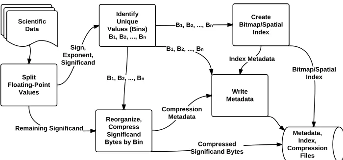
Figure 2.1: Compression methodology, described in Section 2.0.1. The bitmap index is used for compression, while the spatial index is used in query processing.
Figure 2.1 gives a bird’s eye view of our compression methodology. We define a partition
to be a compression stream of bounded maximum size. We define a bin to be a set of values with an equivalent set of high-order bytes. Since we are working under the assumption of highly similar high-order bytes, we expect the number of bins B to be much smaller than the maximum number possible, which is 28k, (65,536 for k= 2). The unique high-order bytes for each partition define the bins that are recorded in metadata. The values in the bin correspond to original floating point values, truncated to the high-order bytes.
For scientific floating point data, we foundk= 2 to be the most effective; it covers the sign bit, all exponent bits, and the first four significand bits of double precision values (approximately two significant figures in base 10 scientific notation). This makes sense, as higher and higher
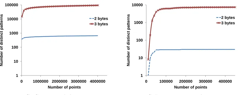
precision in scientific data tends toward high-entropy values or even noise. k= 3, by contrast, has between three and four significant figures. To verify the choice of k, Figure 2.2 shows the logarithm of number of distinct high-order bytes recorded as a data stream is processed. For
k = 2, a very small cardinality is seen relative to the the number of points processed, with the distinct values stabilized after a certain number of data points. The size of the metadata increases proportionally to the total number of bins B. As shown in Figure 2.2, for 2 of the scientific datasets, the size of metadata is less 0.1% of the dataset for k= 2, due to the small number of distinct patterns. Whereas for k = 3, the number of distinct patterns increases by a large factor of 1,000, due to exponential increase in the number of possible values. This
proportionally increases the metadata size. Thus,k= 2 is chosen as a default configuration for ALACRI2TY.
1 10 100 1000 10000 100000
0 1000000 2000000 3000000 4000000
Number of di st inc t pat ter ns
Number of points
2 bytes 3 bytes 1 10 100 1000 10000
0 100000 200000 300000 400000
Number of di st inc t pat ter ns
Number of points
2 bytes 3 bytes
GTS potential dataset S3D temperature dataset
Figure 2.2: Cumulative growth of the number of distinct higher order 2-byte and 3-byte pat-terns for increasing data size. The number of distinct byte patpat-terns is plotted on a logarithmic scale.
values located in each bin corresponds to the floating-point equivalent of the high-order bytes with all zero low-order bytes. Based on the distinct values of High-Order bytes obtained, we
create equality encoded bins. That is, each of the distinct values translates into a bin value. Data points having same High-Order bytes as bin value, belong to that bin. Thus, the
high-order bytes are never stored separately for each data point.
We additionally reorganize the low–order bytes to be contiguous in each bin. These bytes can then be compressed by a general-purpose compressor on a per-bin level. The low–order bytes
could be high-entropic in nature. Thus, before compressing the stream of low–order bytes,
we utilize a simple frequency-counter, tracking the occurrences of each possible byte value. If there is an uneven frequency distribution observed, the low–order bytes are likely to be
compressed well by entropy encoding methods such as Huffman encoding. If an approximately
even distribution is observed across all possible byte values, the compression of the low-order bytes for that particular bin is skipped. ALACRI2TY additionally maintains record of which bins are compressed in the metadata. To maintain the spatial index to bin mapping, we build
a bitmap index that identifies each spatial index with a bin, using size logarithmic of the number of bins. This bitmap can be compressed more effectively if the assumption of similarity
between adjacent values is held, a common occurrence in scientific datasets. The metadata
to the compression includes the high-order bytes themselves and the offsets of each bin in memory/file.
Upon compression, there are three distinct data structures: (1) the compression metadata,
bin-partitioned low–order bytes, which may or may not be compressed.
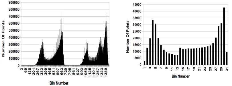
Since our bins are based on distinct values of high-order bytes, the distribution of values within each bin is dependent on the input data. Figure 2.3 shows the bin distribution for two
different datasets. As it can be seen, the distribution of values in bins is uneven. While for
query processing we ideally want equidistributed bins to minimize false-positives, an uneven distribution can also be useful, allowing for a higher compression ratio of the bitmap index.
GTS potential dataset S3D temperature dataset
Figure 2.3: Bin distribution for two scientific datasets.
Lossy Compression
In some cases, the scientific data being stored does not need to be a “pristine” copy. For
instance, some datasets store only a subset of the entire simulation data, throwing out the rest. Others are derived from an approximate mathematical abstraction of a complex physical
phenomenon and do not necessarily correspond to the ideal physical phenomenon. Whatever
the case, lossy compression can be used to cut down drastically on the data. We perform a very simple truncation operation on the low-order bytes, based on a user-defined error level. For
instance, for an error bound of 0.1%, only the most significant 10 bits of significand are needed. Since the most significant four bits are encoded in the high-order bytes, this means that only the next most significant six bits are needed in the low-order bytes, reducing the amount of
low-order byte storage by a factor of over six. Better yet, this truncation operation can easily be dropped into the overall compression process, performing the truncation during the data
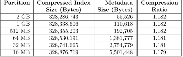
Table 2.1: Compression ratio for different data partition sizes. Original GTS Potential data is 3,414,682,240 bytes (2,561,011,680 low-order bytes).
Partition Compressed Index Metadata Compression Size (Bytes) Size (Bytes) Ratio
2 GB 328,286,743 55,526 1.182
1 GB 328,338,606 110,618 1.182
512 MB 328,355,203 192,705 1.182
64 MB 328,530,191 1,381,777 1.181
32 MB 328,741,665 2,754,779 1.181
16 MB 328,876,719 5,501,448 1.179
2.0.2 Choosing a Partition Size
SinceALACRI2TYis parameterized by the partition size, the choice of such a parameter must be looked at more closely; the number of partitions should be small to minimize the metadata size, but large enough to saturate the parallel file system.
Fortunately, the overall database size is largely independent of the partition size, since the
metadata is much smaller than the raw data and the index size is roughly the same. Table 2.1 shows the bytes used by each component of ALACRI2TY, under varying partition sizes. The difference in overall amount of data used is quite small and the compression ratio of the index data is barely affected, though the rate of growth of the metadata implies that partitions in the
lower megabyte range would begin to suffer. However, since large scientific data sets are the
primary target of our research, we do not expect very small partition sizes to be used.
2.1
Lossless Compression Performance
To analyze the performance of our lossless data compression scheme, we compared the
compres-sion ratios (CR), comprescompres-sion throughput (TC) and decomprescompres-sion throughput (TD) over 20 publicly available scientific datasets [5], against a number of lossless compression utilities such
as FPC[5], fpzip[9], gzip and bzip2. In addition, we tested our method on application datasets
such as Flash [1], GTS [12], and XGC [10]. ALACRI2TY can be used with a compression ra-tio preference or throughput preference. The preference opra-tion given governs which underlying
general purpose compressor (zlib or bzip2) is chosen to compress ALACRI2TY’s index. bzip2 is used to increase the compression ratio at the cost of throughput, while zlib is used to favor
throughput.
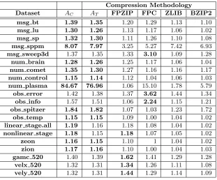
Table 2.2: Compression metrics for various methods, againstALACRI2TY with a preference for compression (AC, using bzip2) and a preference for throughput (AT, using zlib).
Compression Methodology
Dataset AC AT FPZIP FPC ZLIB BZIP2
msg bt 1.39 1.35 1.20 1.29 1.13 1.10
msg lu 1.30 1.26 1.13 1.17 1.06 1.02
msg sp 1.32 1.30 1.11 1.26 1.10 1.08
msg sppm 8.07 7.97 3.25 5.27 7.42 6.93
msg sweep3d 1.37 1.35 1.33 3.10 1.09 1.28
num brain 1.28 1.26 1.25 1.17 1.06 1.04
num comet 1.35 1.30 1.27 1.16 1.16 1.17
num control 1.15 1.14 1.12 1.04 1.06 1.03
num plasma 84.67 76.96 1.06 15.10 1.78 5.79
obs error 1.42 1.38 1.37 3.62 1.44 1.34
obs info 1.57 1.51 1.06 2.24 1.15 1.21
obs spitzer 1.84 1.82 1.07 1.03 1.23 1.72
obs temp 1.15 1.15 1.09 1.00 1.04 1.02
linear stage.all 1.19 1.16 1.18 1.08 1.04 1.02
nonlinear stage 1.18 1.15 1.18 1.07 1.05 1.02
zeon 1.16 1.15 1.10 1 1.04 1.02
zion 1.17 1.16 1.10 1.00 1.04 1.03
gamc 520 1.40 1.39 1.62 1.41 1.29 1.28
velx 520 1.32 1.31 1.34 1.26 1.11 1.08
vely 520 1.32 1.31 1.44 1.29 1.14 1.09
though ALACRI2TY still provides superior compression for 12 out 20 datasets. In terms of throughput, however, the throughput preference gives superior decompression rates on all but
a single dataset, and superior compression rates for 16 of the 20 datasets.
To explain our superior performance on most of the datasets, we argue that the linearized and bin-based compression of the data generally allows a much greater exploitation of existing
compression algorithms than the normal distribution of scientific data that was passed to the
other compressors. The reorganization of the data allowed gzip2 and bzip algorithms to be utilized as best as possible, causing the data to be reduced significantly because of the splitting
Table 2.3: Compression Throughput for various methods, againstALACRI2TY with a pref-erence for compression (AC, using bzip2) and a preference for throughput (AT, using zlib).
Compression Methodology
Dataset AC AT FPZIP FPC ZLIB BZIP2
msg bt 10.78 57.99 41.36 32.16 19.23 4.68
msg lu 10.52 87.96 38.77 28.70 17.57 4.40
msg sp 8.73 57.17 41.52 35.52 18.80 4.49
msg sppm 15.78 56.11 64.98 92.39 77.35 1.91
msg sweep3d 10.45 56.11 46.71 31.64 18.29 4.54
num brain 37.75 84.41 42.58 26.68 17.69 4.42
num comet 14.61 19.03 40.95 23.16 17.13 4.88
num control 22.19 47.21 39.13 22.64 17.50 4.37
num plasma 5.41 82.29 41.52 22.92 28.31 0.79
obs error 31.55 73.80 42.96 22.29 24.21 5.11
obs info 10.74 70.23 41.22 12.37 19.82 4.60
obs spitzer 15.03 21.72 37.98 25.17 18.65 5.76
obs temp 20.57 58.70 38.74 15.93 17.76 4.39
linear stage.all 30.09 59.26 40.72 17.29 17.14 4.38
nonlinear stage 30.97 58.90 40.21 16.94 17.02 4.35
zeon 19.57 49.73 38.20 11.85 18.23 4.42
zion 13.97 54.18 38.43 11.85 18.21 4.43
gamc 520 18.35 19.87 46.72 131.65 20.92 4.80
velx 520 15.74 110.27 47.91 43.55 19.04 4.48
vely 520 73.28 106.01 45.88 47.75 19.14 4.50
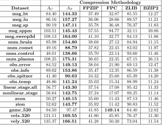
Table 2.4: Decompression Throughput for various methods, against ALACRI2TY with a preference for compression (AC, using bzip2) and a preference for throughput (AT, using zlib).
Compression Methodology
Dataset AC AT FPZIP FPC ZLIB BZIP2
msg bt 84.40 144.33 37.49 32.87 85.55 12.27
msg lu 86.16 157.27 36.06 28.66 89.57 11.21
msg sp 90.19 147.11 35.78 36.48 76.37 11.83
msg sppm 103.51 145.43 57.55 94.77 32.11 39.86
msg sweep3d 108.13 164.00 41.10 32.77 84.13 11.86
num brain 85.98 154.80 38.68 27.12 84.94 11.15
num comet 49.16 88.79 37.82 22.45 83.02 11.97
num control 48.01 138.66 35.70 22.14 93.60 11.46
num plasma 108.25 175.31 36.65 22.35 67.15 26.13
obs error 84.52 149.13 38.04 21.90 69.13 12.47
obs info 89.02 153.86 35.47 12.35 86.59 11.38
obs spitzer 41.40 90.63 34.32 25.68 65.39 14.20
obs temp 48.86 141.24 35.03 15.34 88.99 11.24
linear stage.all 56.77 143.30 37.54 17.08 95.42 11.33
nonlinear stage 56.64 142.75 37.24 17.07 89.25 11.14
zeon 50.27 140.15 35.60 11.43 87.13 11.46
zion 52.62 143.77 35.92 11.42 90.83 11.52
gamc 520 94.50 97.47 41.85 149.14 64.40 12.82
velx 520 121.11 169.55 41.80 45.85 76.47 11.30
Chapter 3
Univariate Query Processing
3.1
Index Generation
The compression methodology presented in Section 2.0.1 is, as shown, efficient for improving the compression ratio of many scientific datasets, but is not optimized for query processing.
Were a range query to be performed using our presented compression index, the entire bitmap
would need to be traversed to map the binned data back to spatial regions. Thus, at the cost of additional storage, we optimize for range queries by using an alternate index which directly
maps spatial indices to data point per bin. This is nothing but inverted index with bins as
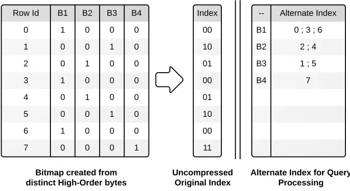
keys. Figure 3.1 shows an illustration of the original compression index and the new bin-based spatial index.
Rather than create a global spatial region-to-bin bitmap, we reorganize the spatial indices by bins to create a bin-based value-to-spatial index mapping. See Figure 3.1 for an example. This organization is advantageous for range query processing, because we now access the spatial
indices by bin, the same as accessing the low-order bytes. The organization is disadvantageous because of the increased space, both for the index itself as well as the additional metadata, such
as file offsets, needed to access the new index. This means, for a partition size ofN elements, approximately NlogN space is needed to store the index, with marginally additional space to store metadata such as elements of a partition within a bin. Therefore, using a maximum
partition size of 232 elements, the index is close to exactly 50% of the raw data size, assuming double precision.
Original index has a mapping from spatial index to which bin the corresponding point
belongs to. Thus, as described before, logB bits are needed per data point. This is a very compact representation, thus helping in compression. But, for efficient query retrieval, we propose an alternate index that lists the Region Ids lying within each bin contiguously. Consider
Figure 3.1: Building a spatial index for query processing, compared to the compression index. Row Id corresponds to a spatial index within a partition.
bitmap index is shown. The alternate index generated is nothing but list of spatial indices
falling under that bin. For example, bin B1, data points at row id 0, 3 and 6 belong to B1. Thus, in alternate index, we store list [0,3,6] corresponding to Bin B1. Thus, alternate index indicates position of ’1’ in original bitmap column for each bin. Please note that within each
Bin, the Row Ids listed are sorted.
This is an alternate way of representing bitmap. With this representation, we need not go
through entire bitmap to retrieve spatial indices for bins of interest. For example, if a query
touches bins B1 and B2, we can directly fetch the spatial indices for values belonging to these bins. Additionally, we maintain a metadata for offsets into this alternate index structure. An
offset pointer to start of each bin’s list is maintained, for efficient seek to the bins of interest.
This offset is obtained from the No. of data points belonging to each bin, which is already captured in Metadata during compression.
As described before, in the compression phase, we reorganized values belonging to by bins
together and compressed Low Order bytes for each bin. With this, alternate index, a direct mapping from each value to spacial index is generated. Thus, region and values both can be
<N number of partitions>
<Metadata offset for partition t> (0≤t < N) <Index offset for partition t> (0≤t < N) <Compression offset for partition t> (0≤t < N) (Repeat for 0≤t < N)
<M number of elements in partition t> <B number of bins>
<Number of elements in bin b> (0≤b < B) <Bin bound b> (0≤b < B)
<Compression offset b> (0≤b < B) (End Repeat)
Figure 3.2: Metadata file format.
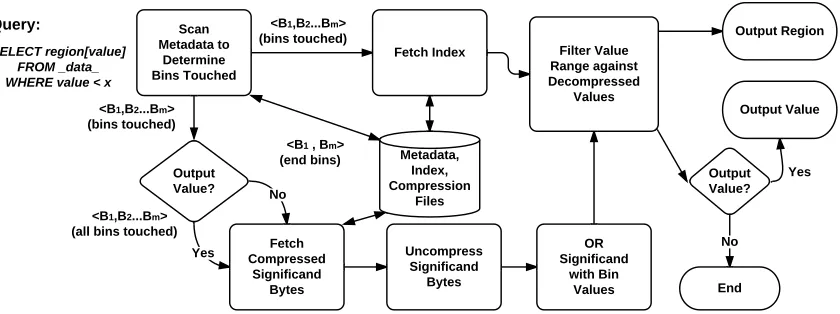
Figure 3.3: Query processing methodology, taking into account metadata, index, and compres-sion data fetching and aggregating.
3.2
Query Processing: File Layout
We split the data used by the query processing engine into three components: a metadata file,
an index file, and a compression file, each corresponding to its purpose described in the previous sections. The metadata file is shown in Figure 3.2.
The metadata file contains partition information, including file offsets for each partition and
bin, the number and bounds (high-order bytes) of bins, and the number of values per bin per partition. The index file and the compression file contain the spatial indices and compressed
low-order bytes, respectively.
3.2.1 Query Processing: Range Queries
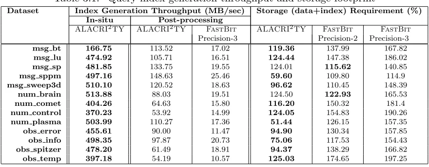
Table 3.1: Query index generation throughput and storage footprint
Dataset Index Generation Throughput (MB/sec) Storage (data+index) Requirement (%) In-situ Post-processing
ALACRI2TY ALACRI2TY FastBit ALACRI2TY FastBit FastBit
Precision-3 Precision-2 Precision-3
msg bt 166.75 113.52 17.02 119.36 137.99 167.82
msg lu 474.92 105.71 16.51 124.44 147.38 186.02
msg sp 481.85 133.75 19.55 124.01 115.62 140.85
msg sppm 497.16 148.63 25.46 59.60 109.80 114.9
msg sweep3d 510.10 120.52 18.63 96.62 110.45 148.39
num brain 513.88 88.03 19.51 124.50 122.93 165.53
num comet 404.26 64.63 15.80 116.20 150.32 181.4
num control 370.23 53.92 14.99 124.05 154.83 190.26
num plasma 503.99 110.27 17.36 51.44 126.15 157.35
obs error 455.61 90.00 11.47 94.90 130.34 157.85
obs info 498.35 97.87 20.73 75.06 117.53 154.43
obs spitzer 478.20 61.49 18.91 94.37 138.29 166.82
obs temp 397.18 54.19 10.57 125.03 174.65 197.25
partition, relevant bins are identified using a method such as binary search, using the high-order
bytes as a lower bound of each bin. Given a non-decreasing order of bin organization in file, for each partition, we need a single seek in the index and the compression file to get to the values
associated with bins of interest. The low-order bytes and spatial indices are read, decompressed,
and reconstructed into the original values, filtering out the ones that do not match the query. In case of queries requesting only spatial regions, all values need not be reconstructed. Thus,
only the end bins are checked for query bounds. For queries requesting values, the values for all bins are fetched and decompressed.
3.3
Results And Discussions
3.3.1 Experimental Setup
We performed our experiments on the Lens cluster on Oak Ridge National Laboratory that is dedicated for high-end visualization and data analysis. Each node in the lens cluster is made
up of four quad-core 2.3 GHz AMD Opteron processors and is equipped with 64GB of memory.
All experiments were run with data located on the Lustre filesystem.
Index Generation
Indexing is a crucial process in the enabling of fast and efficient query processing. However,
index generation is a very time and storage intensive step for large scientific datasets. For this reason, it is crucial that the indexing technique thatALACRI2TYutilizes provides both speed and storage improvements in order to be relevant in future scientific analysis and simulation
on 13 scientific datasets and gathered throughput and storage-related metrics. Table 3.1 shows
the results that we obtained from these experiments. For all 13 datasets, our indexing strategy provides a throughput several times higher than that offered by FastBit[13]. On the storage
front, ALACRI2TY’s total footprint, consisting of both index and data, is significantly less than FastBit with precision-3 binning on all of the 13 datasets, and less than FastBitwith precision-2 binning on 11 of the 13 datasets. For the other two datasets (msg sp and num -brain), we require slightly more space than FastBit with precision-2 binning. Furthermore, our method is parameterless, and its ability to provide high-throughput in the index generation process makes it ideally suited forin-situ index building, visualization and analysis routines.
3.4
End-to-End Query Performance Evaluation
For a comparison of end-to-end query performance, we perform queries under a number of
scenarios. First, we look at variable-centric queries, that is, queries returning the actual values of variables, as opposed to just the spatial regions. Second, we look at region-centric queries,
that is, queries returning the spatial regions corresponding to variables of interest. We compare
each of these types of queries againstFastBitwhich utilizes bitmap index and sequential scan of data. We also compared our performance with MonetDB[2], a popular column-store database
system. However, the performance for MonetDB was about two orders of magnitude slower than
ALACRI2TYfor the queries tested, and is thus not included. We also did not compare against SciDB[3], another popular scientific database system, as it does not yet maintain any form of
index, making queries with variable constraints equivalent to sequential scan.
We used following two scientific simulation datasets to evaluate our query performance in terms of value centric queries and region centric queries.
1. GTS data(GTS)[12]: A particle-based simulation data for studying plasma
microturbu-lence in the core of magnetically confined fusion plasmas of toroidal devices.
2. The S3D data(S3D) [7]: It is first principles based direct numerical simulation (DNS)
of reacting flows which aids the modeling and design of combustion devices in nuclear reactors.
3.4.1 Variable-Centric queries
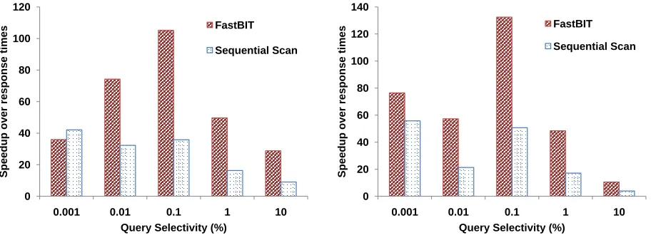
Figure 3.4 shows speedup in value-based query response time using our method, compared to FastBit’s default and precision-based indexing, with varying query selectivity. By query
selectivity, we refer to the percentage of the raw dataset returned by a query. For two scientific
0 20 40 60 80 100 120
0.001 0.01 0.1 1 10
Speedup over
r
esponse
ti
mes
Query Selectivity (%) FastBIT Sequential Scan 0 20 40 60 80 100 120 140
0.001 0.01 0.1 1 10
Speedup
over
response
ti
mes
Query Selectivity (%) FastBIT
Sequential Scan
GTS potential dataset S3D vvel dataset
Figure 3.4: Comparison of speedup of ALACRI2TY overFastBit, and sequential scans, for variable-centric queries when the query selectivity is varied from 0.001% to 10.0%.
needed by our method as opposed to FastBit. However, with FastBit’s Order Preserving
Bin Based Clustering (OrBic) option [14], the values are clustered together per bin, similar to our method. As opposed to OrBic, our method needs only read compressed low order bytes
from disk. Thus, the amount of data fetched from disk is less than 75% of actual data size
with respect to selectivity, thereby reducing the I/O read time. FastBitmainly introduced the OrBic technique forcandidate checks in region-centric queries. For value-centric queries, giving this option seemed to evaluate based on the original data only, giving behaviour similar to
default binning. Moreover, the storage requirement for OrBic limits the number of bins used to be less than 100, which increases the number of values to be fetched per bin. For these reasons,
we compared value query response times with FastBit’s precision binning option, which for
our applications was the best performing, and default binning as a baseline.
For value-centric queries, not much difference is observed in the response time by FastBit
using precision binning and default binning. This is because, in both cases, random disk access dominates processing time. While FastBit has a very CPU processing time for each query,
the I/O time spent on random file access dominates the overall query response time.
The speedup observed increases from factor of 35 for 0.001% selectivity to 105 for 0.1% selectivity. Here the performance improvement is solely due to significantly less number of
seeks. On increasing query selectivity, FastBitcan fetch more consecutive blocks of file from
3.4.2 Region-Centric queries 0 1 2 3 4 5 6 7 8 9
0 500000 1000000 1500000 2000000
Query Re spo nse T im e (seconds )
Number of hits
FastBIT with 1 million bins
ALACRITY
FastBIT with precision = 3
0 0.2 0.4 0.6 0.8 1 1.2 1.4 1.6 1.8 2
0 1000000 2000000 3000000 4000000
Qu ery response ti me (se conds)
Number of Hits
ALACRITY
FastBIT with precision = 3
GTS potential dataset S3D vvel dataset
Figure 3.5: Comparison of response return by FastBit against ALACRI2TY for region-centric queries with varying number of query hits.
Figure 3.5 shows region query response time with varying number of hits (records returned)
for our method compared to FastBit with precision and default binning. For region-centric
queries, only the points falling within misaligned bins need to be evaluated. ForFastBit, the type of binning used plays a definitive role in determining the time taken to respond to region
queries. In the case of precision binning for FastBit, it can answer queries involving three
decimal point precision by going through the bitmap alone. It need not seek to the disk if the range specifed in the query involves less than three decimal points. On the other hand, the
default binning option needs to perform raw data access to evaluate edge bins.
The performance of our method is better than the precision binning in many cases, but the non-regular distribution of bins, as shown in Figure 2.3, causes spikes in performance. This
happens when misaligned bins happen to be those with the largest number of points contained
in them. In these cases, disproportionally more values are read and decompressed than the typical case (i.e. high false positive rate), causing it to be slower than FastBit.
3.4.3 Needle in a Haystack Experiment
First, we will consider a so-called “the needle in a haystack” experiment, where a needle (or 1% of a 6 GB dataset) is being placed into a growing size haystack (6 GB, 100 GB, 500 GB, and 1
Table 3.2: Response time (sec.) for the needle in a haystack experiment. ALACRI2TY used a 64 MB partition size.
Size Partition ALACRI2TY Sequential Sequential
Count Response Total I/O Read
6 GB 96 6.4 21.4 14.0
100 GB 1600 7.4 280.8 225.1
500 GB 8000 7.8 1,364.6 1,081.9
1 TB 16384 7.8 2,712.5 2,170.8
at relatively constant cost; and (2) to get a feel for a potential of or a lack of using parallel I/O approaches to read the entire data (i.e., full data scan) while searching for the needle. Basically,
we address the following intriguing question: Could parallel I/O potentially eliminate the need
for database indexing and query processing offered byALACRI2TY? Instead of actually using a parallel I/O read of the entire data, we perform a sequential scan and assume an ideal scaling
of a parallel I/O library to avoid a plausible argumentation in favor of or against a particular
parallel I/O library implementation.
We consider a univariate query type for this experiment. Table 3.2 clearly demonstrates
that (1) ALACRI2TY is quite robust, namely, increasing the size of the haystack does not affect the response time for retrieving the needle; and (2) matching ALACRI2TY’s response time for a 1 TB dataset would require more than 300 parallel I/O readers with an ideal scaling,
and likely 30,000 readers for a 100 TB data set.
3.4.4 Performance analysis
Figure 3.6 shows the breakup of overall processing time into I/O and compute components,
corresponding to index/bin loading and decompression, respectively. The dataset tested on is
S3D using the velocity variable. I/O is still a significant portion of the time, but much of the overall time is spent decompressing the data. Combined with the superior performance in many
cases compared to FastBit, we believe that the portion spent on decompressing is a positive
aspect of our system, as it takes much of the pressure off of I/O operations, which is certainly good for performance in HPC contexts. Furthermore, this opens up windows for performing
clever optimizations, such as multithreading I/O and decompression to hide the compute time,
0 10 20 30 40 50 60 70 80 90 100
0.001 0.01 0.1 1 10
T
im
e
spent
(%
)
Query Selectivity (%) I/O CPU
0 10 20 30 40 50 60 70 80 90 100
0.001 0.01 0.1 1 10
T
im
e
Spent (%
)
Query Selectivity (%) I/O CPU
Chapter 4
Multivariate Query Processing
4.1
Challenges and Strategies
ALACRI2TY, in its original incarnation described in previous chapter, was only considered for univariate queries requesting spatial regions and variable values. In this chapter, we extend
ALACRI2TY to handle a wider range of multi-variate, multi-dimensional query types. To address these aspects using ALACRI2TY, a number of technical challenges need to be dealt with. A significant challenge lies inALACRI2TY’s rearrangement of the low-order bytes by variable value, inherent in the compression/binning process. While the reordering allows
highly efficient query processing on variable constraints,ALACRI2TYloses the ability to per-form random value access with respect to spatial indices. Therefore, the lookup of binned values
based solely on spatial index must be a lightweight operation on the binned indices.
Further-more, an efficient aggregation of intermediate results must be provided, as the spatial indices in each bin are not bitmap-based and do not enjoy the benefit of efficient logical operations.
ALACRI2TY addresses these challenges by casting the multi-variate queries into multiple range queries with univariate constraint and efficiently aggregating each constraint, described
in Section 4.2.
To provide fast partial result aggregation, we perform on-the-fly bitmap generation of partial spatial regions. Finally, we map the resulting spatial regions into the bins using an efficient
list-intersection method and retrieve the values.
4.2
Heterogeneous Query Process
4.2.1 Overview
Figure 4.1: Overview of ALACRI2TY Query Processing Engine, on a per-partition level. Input Q is a query of the form (SR,SV,VC,DC), where SR→select region (X, Y), SV → list
of variable values to retrieve (for example, Select region, [V1]),VC →list of variable constraints
each variable. Figure 4.1 presents an overview of end-to-end query processing for various query
types on ALACRI2TY compressed data, specifically for queries on multi-variate constraints. Note that, for this chapter, we assume that the result variable is different from the constraint
variables; this represents the worst case of not being able to cache previously read results.
Given an input query, with variable constraints (VC) and dimension constraints (DC), a
number of operations are performed:
• Each variable constraint is evaluated independently using univariate range-query
process-ing. This results in a list of spatial regions for each variable constraint.
• Results from each variable constraint are combined based on the logical operators to obtain
a final sorted list of spatial regions. This is described in more detail in Section 4.2.2.
• If dimension constraints are specified, the resulting set of spatial regions are pruned
ap-propriately.
• Finally, if there are any variables requested, then each spatial index must be mapped to
its corresponding bin for the variable requested, due toALACRI2TY’s reorganization of data. We call this mapping theBin Partitioner, and it is described in Section 4.2.3. The actual reading of variables depends on the level of detail requested, see Section 5.2.
Overall, we show a multi-fold higher performance than the state-of-the-art SDBMS systems on multi-variate query types, with a total storage bound of less than 135% of the original data
size, and no need for storing the original data.
4.2.2 Multi-variate Constraint Processing
For constraints on multiple variables, each variable constraint is evaluated usingALACRI2TY’s univariate query processing. The resulting spatial region list obtained from each variable
con-straint must be combined to give final output of spatial regions satisfying the given concon-straint.
Query planning is not considered but is planned to be included for further query optimization. To formalize, a query consisting of v variable constraints would returnv spatial region sets Ri, for 1≤i≤v. Each set consists ofbi disjoint sorted lists of spatial indices, one for each bin
touched during the query. Call these listsSi,j, for 1 ≤j ≤bi. There are two goals here. The
first is to produce a sorted list of indices, over all bins, for each variable constraint. The second
is to combine the variable constraints using the logical operators in the query.
There are two ways to accomplish the first goal: (a) merely sorting the lists, or using a
multiple-list-merge algorithm, or (b) utilizing a bitmap over the spatial region in question, and
setting bits iteratively least-to-greatest to maintain cache locality.
The bitmap aggregation algorithm is shown in Algorithm 1. In order to make the aggregation
and scan the front of each bin. If the index at the front of the bin list lies in the block, the
bit is set, and the next element is examined. Using the bitmap representation is efficient for combining results with other variable constraints because of fast logical operations.
Algorithm 1: Spatial bitmap generation—aggregation of sorted lists input :B – number of bins
input :bi – size of bini(1≤i≤B)
input :Si – sorted spatial region lists (1≤i≤B)
output:M – spatial region bitmap
1 Maintain high cache hit-rate (bit-wise)
2 block←8×cache line size
3 offsets←B-length array, initialized to 0 4 forblk∈ {0,block,2×block, . . .}do
5 forbin∈ {1,2, . . . , B}do
6 Set next index bit if within our cache unit?
7 while Sbin[offsets[bin]]≤blk+block 8 and offsets[bin]≤bbindo
9 set bit inM atSbin[offsets[bin]] 10 offsets[bin]←offset[bin] + 1 11 end
12 end 13 end
If we use the bitmap representation to aggregate intermediate results, then we must also
consider mapping the bits back into spatial indices for output. Thankfully, this can also be a
fast operation. Operating at a byte granularity, we compute a lookup table for each possible byte-to-index mapping. That is, we precompute the offsets of spatial indices on a byte level
and scale appropriately. This can be done at database initialization and takes insignificant time
compared to the query process as a whole.
4.2.3 Spatial Index Bin Partitioner
For queries requesting variable values, the spatial index results must be mapped to their residing
bins with respect to the new variable. As discussed, we must do this because ofALACRI2TY’s compression/indexing, which shuffles the data into bins. The Bin Partitioner reads the index of each bin and performs an intersection operation between the list of binned indices and the
intermediate results, generating a list of offsets of values to be read from the bin. The output of this operation is a list of bins that contain values satisfying the query constraints and offsets
to those values.
Figure 4.2: High-level overview of the Bin Partitioner that divides the given sorted list of spatial indices into multiple lists of bins touched based on the alternate index, with an example.
read from each bin, the spatial indices in question are partitioned into their corresponding bins,
taking into account within-bin offsets for reading, as well as value counts for bookkeeping
purposes. In short, list intersection operations must be performed between the input list and each bin-level list.
To perform these intersections efficiently, there are two methods we consider, both of which
take advantage of the sorted nature of the respective bin lists and input list. First, we consider simply building a reverse index, making a list on the order of the partition size and explicitly mapping spatial indices back to bins. While there is a high cost memory-wise, it only requires a
single pass of the binned indices in file and the input list. Second, we consider atwo-way binary search to traverse the lists and find their intersection, which uses little additional memory. The primary benefit of the algorithm is that the input spatial indices are likely much different than
the indices in each bin, allowing the binary search on both lists to “skip ahead” in the list. Algorithm 2 describes the process of the “back-and-forth” searching for intersected items. Not
listed in the algorithm is the additionally recorded offsets and bin counts, though these are
read/computed at negligible additional cost. Since the spatial indices are partitioned among the bins, we expect a large amount of list pruning through this method.
Regardless of the method used, the output of the Bin Partitioner is a list of bins with the prerequisite spatial indices as well as the offsets of values to fetch. The corresponding bins are fetched from disk and (if necessary) decompressed. After recombination with the high-order
bytes, the resulting spatial indices and variables are returned. In order to minimize the disk
Algorithm 2: List intersection using binary search input :L1, L2 – input lists
output:I – intersection list
1 x1←1current position in L1
2 x2←1current position in L2
3 while x1≤ |L1|andx2≤ |L2|do
4 PruneL2 to first position≥item atx1
5 b2←binary search(L1[x1], x2,|L2|) 6 Check for equality
7 if L2[b2] =L1[x1]then 8 appendL2[b2] to I
9 b2←b2+ 1
10 end
11 PruneL1 to first position≥item atb2
12 b1←binary search(L2[b2], x1+ 1,|L1|) 13 Check for equality
14 if L1[b1] =L2[b2]then 15 appendL1[b1] to I
16 b1←b1+ 1
17 end
18 Update list positions
19 x1←b1
20 x2←b2+ 1
Table 4.1: Parameters influencing query response time.
Parameter Description
NP Number of data points in each partition
N Total data points
P
Number of partitions to scan in query
P≤ N
NP, with equality if
no dimension constraint in query.
M Number of variables in query
σi Query selectivity for each variablei(i= 1. . . M) (Predicate selectivity)
π Overall query selectivity
tseek Cost of random seek on disk
RIO Disk I/O read rate for small data read
RLargeBlockIO Disk I/O read rate for large block data read
RD Decompression rate in bytes/s
SData Size of original dataset
(N×8 for double precision datasets)
K Average time for 1 read/write from memory and perform operation in CPU
4.2.4 Cost Analysis
Given the overall query processing methodology discussed in the previous sections, we can
anal-yse the cost of each operation and its contribution to the query process as a whole, given some
information on the hardware characteristics (e.g., seek costs) and on the relationship between data, database layout, and query patterns. These parameters are shown in Table 4.1. Query
planning has not yet been enabled by our technology, but our model would be sufficient for
performing such planning, by utilizing the compression metadata and providing some additional statistical data to estimate the selectivity parameters, something which has been well-studied
in the literature.
As described, query processing is based on the following components, which we will analyse
separately:
• Time to evaluate region queries for each variable specified in constraint (TU),
• Time to combine results from each univariate constraint evaluation (TC), and
• Time for value retrieval of the specified variable in select clause, if applicable (TV R).
The overall elapsed time during query processing, assuming a single variable requested as
Computing TU
The cost for univariate region query processing involves reading the spatial indices within query
bounds as well as low-order bytes for bins not entirely in the query bounds, for each partition.
A small portion of time is spent in reconstructing the values in the out-of-bounds bins and evaluating against the constraint. This, however, is small enough with respect to total time to
be ignored when approximating query cost.
The univariate query processing time is dominated by the I/O overhead. ALACRI2TY therefore tries to minimize the number of I/O operations performed. There are two seeks and
data reads at the bin-level, when evaluating the constraints on boundary bins, or those whose range of values straddle the constraint. Exactly one seek is needed for spatial index retrieval, making a total of 3 seeks for each partition. In addition, there is a sequential read for the index
which is 50% of the equivalent raw data being retrieved, for double-precision data sets. This is a large block of data read, thus, data transfer rate isRLargeBlockIO.
TU =P×(3×tseek) +σi×0.5×
SData RLargeBlockIO
(4.1)
As can be seen from Equation 4.1, the univariate query processing time grows both with the
partition count through seek costs, and with the proportion of the amount of output through read costs. Thus, for serial query processing, we ideally want to minimize the partition count
to minimize the number of seeks. Also, since the amount of I/O grows with the selectivity
rather than with the raw dataset size, the univariate query processing is expected to scale to progressively larger datasets, though query planning is needed for highly lopsided variable
selectivities.
Computing TC
The cost of aggregating univariate results includes the cost of in-memory bitmap creation and merging each variable involved in the query, as well as converting the final answer to a list form
for output. For each variable, the number of bits that need to be set in bitmap is proportional
to the query output. Merging these bitmaps requires a pass over N values for M variables, giving a time complexity of O(M N), though the constant associated with the actual time in this step is very small due to cache conscious bitmap creation. Finally, converting to list form
Table 4.2: Parameters for value retrieval estimation. Parameter Description
B Total number of bins for variable to be retrieved
bi Size of bin i(i= 1. . . B)
φ Query selectivity for partition
nf etch Number of bins to fetch
bmax Size of the largest bin
C Fraction of total bins compressed
TC =KN M X
i=1
σi (bitmap setting)
+KN M (bitmap merging)
+KN π (list conversion) (4.2)
Compared to the other steps in the overall query processing, this step is a complete in-memory operation, and takes a lesser portion of time with respect to the I/O operations.
Computing TV R
In the case of solely region retrieval queries, this step does not need to be performed. However,
if a variable value is requested as output, then the overall value retrieval time TV R is split
into componentsTBP andTV F, whereTBP represents theBin Partitioner and TV F represents
the retrieval of the low-order bytes. The former includes reading the index of each bin and
performing the partitioning, and the latter includes seeking to and reading the low-order bytes in each bin. The additional parameters needed for this estimation are given in Table 4.2.
Overall, TV R =TBP +TV F.
In the Bin Partitioner, the reading of the index is a fairly straightforward operation, but the partitioning itself requires some analysis. The worst case time complexity of intersection by
two-way binary search for lists of sizemandnisO(mlog(n) +nlog(m)), when the lists contain the exact same indices. In practice, there is a large degree of variability between the two lists,
so this level of performance is rarely seen. Overall, there are b intersections performed. The size of the resulting list ism=φ×SP.
Using the fact that PB
TBP = B X
i=1
(bi×log (φ×SP) +φ×SP ×logbi)
≤SPlog (φSP) +φBSPlog (bmax)
≈φBSPlog (bmax) (4.3)
When the Bin Partitioner step is performed, the within-paritition selectivity (φ) is already known. Using this information, we can choose which partitioning method to use, using two-way binary search for small selectivities, and the in-memory forward index method for higher
selectivities, which involves 2 passes over the partition (SP). The two-way binary search is used
when, givenφ, the inequality
φjBSPlog (bmax)<2×SP (4.4)
holds.
This step also involves, reading in the index of the variable being retrieved (50% of data size for double-precision data sets). This is again a large block read. Thus, combining the
worst-case performance of the parititioning operation with the index reads, the overall bin-partitioning
time is:
TBP = 0.5×
SData RLargeBlockIO
+ 2KN. (4.5)
The output after bin partitioning is a set of nf etch bins to be fetched. The remaining
processing involves a single seek and read for each bin touched. The overall time for value retrieval is thus given by:
TV R= 2×KN + 0.5×
Data RLargeBlockIO
+nf etch( tseek
2 +
bmax RIO
+Cbmax RD
) (4.6)
This step tries to combine several random disk reads into a single seek and read operations
using Bin Partitioner. On an average only half of random seeks are needed fornf etch. Thus,
cost of value retrieval is improved compared to other query processing schemes as shown in the
following section.
The overall query processing performance depends on all three of the above components mentioned. Table 4.4 shows the cost model based and actual query response timings for 1
partition. The hardware and data parameters used are shown in Table 4.3. The hardware
Table 4.3: Hardware and data parameters used in cost model.
Parameter Value
P 1
RIO 60 MB/s
RLargeBlockIO 300.96 MB/s
K 8.78E-9
N 250000000
NP 250000000
SData 2000000000
RD 150 MB/s
Tseek 0.011 s
Table 4.4: Cost model-based and actual response timings. Variables σ per Estimated TU TC TV R Total
variable or Actual
2 1% Estimated 0.38 0.23 16.47 17.08
2 1% Actual 0.43 0.16 15.64 16.61
3 1% Estimated 0.58 0.41 18.95 19.94
3 1% Actual 1.42 0.22 16.99 18.84
2 10% Estimated 3.24 1.04 18.95 23.23
2 10% Actual 1.67 0.68 18.84 21.66
3 10% Estimated 4.87 1.61 18.95 25.43