On the sensitivity analysis of dynamic characteristics for structural modification

ON THE SENSITIVITY ANALYSIS OF

DYNAMIC CHARACTERISTICS FOR

STRUCTURAL MODIFICATION

Aminudin Hj Abu

Mohd Azmi Yunus

Muhamad Norhisham Abdul Rani

Nor Azizi Othman

1.0 INTRODUCTION

linear combination for non-modified structure amount of changes of an eigenvector and determined the sensitivity coefficient from the normalised mass and orthogonal condition and calculated the change rates for the first eigenvector. Wang[5] applied mode summation technique of accelerated mode on the sensitivity analysis and improved the estimation accuracy. Min, Hyun-Gi et. al.[6] used direct differential method and studied the kinematics of an automobile suspension system with the sensitivity analysis. The sensitivity analysis methods explained above are widely used by most of the researchers; however none of them considered the sensitivity analysis can determine the location of the modification and the modified value, but the analysis itself is a key problem. Once the modifications are made, the structure correspondently changes the natural frequency and the result may not be the optimum value. For instance, if we intend to change the original structure but with less modified points and less subsequent on the dynamic parameters in achieving the desired value, what should we do?

1.1 THEORY

1.1.1 DYNAMIC CHARACTERISTICS OF STRUCTURE CHANGES

The equation of motion in a general vibration system with harmonic excitation is expressed as follows

[ ]M{ }&x&+[ ]C{ }x&+[ ]K{ }x ={ }F( )t (1)

where,

[ ]M is a mass matrix,

[ ]C is a damping matrix,

[ ]K is a stiffness matrix, ( )

{ }F t is a force vector,

{ } { } { }x, x&, x&& is displacement, velocity and acceleration.

When the structure changes, the mass, damping and stiffness change correspondingly. The equation for the changing structure can be written as

[M+ΔM]{ }&x&+[C+ΔC]{ }x&+[K+ΔK]{ }x ={ }F( )t (2)

here, ΔMis the mass change value, ΔC is the damping change

value and ΔKis the stiffness change value. Taking the Laplace

transforms for equation (2) one finds

[ ] [ ] [ ]

(

s2M+ΔM +sC+ΔC + K+ΔK

)

{X( )s}={F( )s} ₍₃₎

Considering the linear transformation {X(s)}={Y(s)}[ ]φ and pre-multiplication both side by

[ ]

_φT_{, then, equation (3) becomes}

(4)

[

] [

] [

]

where,

A linear relationship exists in the equation (4) and

( )

{ }Y s ₌

[ ]

_φ*{ }Z( )s (5)

where,

From equation (3) and (5) one will get

or

[ ] [ ] [ ]

(

s2Mm ₊sCm ₊ Km

)

{ }Z( )s ₌

[ ]

_φ T{F( )s}

(6)

Here,

[ ]

m

M ,

[ ]

Cm and

[ ]

Km are diagonal matrices.

Equation (6) is a new modal model. The new mode shape matrix of a new structure becomes

(7)

Modal parameters

[ ]

_Mm ,

[ ]

_Cm ,

[ ]

_Km and [ ]_φ can be obtained from

the modal analysis of the original structure, then, a new modal model after modification can be built. A linear transformation by new structure modal matrix is

[ ]

_φ

[ ]

_φ* [ ]_{φ =}

[ ]

_φφ* ⎥⎦

⎤ ⎢⎣

⎡

= T T T

[ ] [

][ ] [ ]

[ ] [

][ ] [ ]

[ ] [

*

][ ] [ ]

* * * * * m m m T m m m T m m m T K K K C C C M M M = Δ + = Δ + = Δ + φ φ φ φ φ φ

[

]

[ ] [ ][ ]

[ ]

[ ] [ ][ ]

[ ]

[ ] [ ][ ]φ φ φ φ φ φ K K C C M M T m T m T m Δ = Δ Δ = Δ Δ = Δ

[ ] [ ] [ ]

( )

{X s}=

[ ]

φ { }Z( )s (8)

Substituting (6) into (8), it yields

(9)

where,

: frequency response between points p and q

1.1.2 SENSITIVITY OF NATURAL FREQUENCY

The relationship between natural frequency and modal mass _Mm_,

modal stiffness _Km _is

(10)

where ,_Mm _{and K}m _{are diagonal matrices, and}

(11)

The sensitivity of natural frequency with respect to structure parameters is the partial differential of with respect to .

1.1.3 SENSITIVITY OF FREQUENCY WITH RESPECT TO MASS

From equation (10) one knows

( ) _{( )}( )

[ ] [ ]

(

)

[ ] [ ] [ ]

(

)

‡”

2 N r r m r m r m r q p p q pq K C s M s s F s X s H + + = = φ φ

( )s Hpq 2 n ω

[ ]

{ } [ ]{ }

[ ]

{ }φ [ ]{ }φ φ φ K K M M T m T m = =

[ ][ ] [ ]

m m n M K

ω2 =

2

n

ω

2

n

ω Pm

[ ] _{[ ]}

_{[ ] [ ]}

i m m n i n M M K M Ý Ý 2 1 Ý

Ý _ω -1 -1

ω

=

m

(12) From equation (11)

(13)

Where is a diagonal matrix composed of modes of the point i.

The inverse matrix differentiations are

or

(14)

The sensitivity of the _ith _{natural frequency with respect to the} th

i mass point is related with the and the _ith _{mode only.}

Therefore, the mode accuracy of the modified point is important.

1.1.4 SENSITIVITY OF NATURAL FREQUENCY WITH RESPECT TO STIFFNESS

From equation (10) and equation (11)

(15)

For matrix

(16)

[ ]

_{[ ] [ ][ ]}

_{[ ]}

2

Ý Ý Ý Ý ni i T i m M M M

M _{φ φ φ}

= =

[ ]

2

ni

φ

[ ]

-1

_{[ ] [ ][ ]}

-1 -1

Ý Ý Ý Ý m i m m i m M M M M M

M ₌₋

2 4 1 Ý Ý ni n i n M

f _ωφ

π

− =

[ ]

_{[ ]}

[ ][ ]

Substitutes (16) into (15)

(17)

1.1.5 FREQUENCY RESPONSE SENSITIVITY

We know that

(18)

here, is the frequency response matrix and

[

Z

( )

jω

]

is the

impedance matrix. Therefore the frequency response sensitivity in terms of partial differential equation or with respect to physical parameters is

.

From equation (18), one can obtain:

(19)

1.1.6 APPLICATION EXAMPLE

Fig. 1.1 is a simple 3 Degree of freedom (DOF)s lumped mass model to be used for the application example for the proposed method. With reference to figure 1.1, five cases were investigated. Case 1, the mass at M1 was added with 0.398kg, case 2 the mass at M2 was added with 0.398kg, case 3 the stiffness was added at K3 with 1.1kN/m, case 4 the mass are added at M3 with 0.398 kg and 0.191 kg respectively and for case 5 the stiffness was added at K2

[ ]

2

2 1 ni n ij K K _φ ω = ∂ ∂ ( ) [ ] [ ( )] ( )

[Z j ] ( ) [ ]j M j [ ] [ ]C K j Z j H + + = = ω ω ω ω ω 2 1

-( )

[

H jω

]

( )

[ _{] [ ] [ ][ ]H}

with the amount of 1.79 kN/m. The sensitivity of the natural frequencies was determined at each case.

Figure 1.1 Simple 3DOFs model

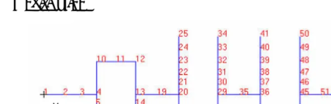
Fig. 1.2 shows the model of a crankshaft system to be used in the proposed method. The process of determining the natural frequencies sensitivity is performed as in previous procedures. In case 1, an additive mass was added to point 35 with 0.5kg. where as, in case 2, a 1 kg mass was added to point 1. In case 3, a 1 kg mass was added to point 71. However, in case 4 and 5, a 1.5 kg mass and 2x103N/m was added to point 71 respectively. The increments of masses and stiffness were added vertically in y-axis. The selected point in each case at the position chosen is to gain the instructive effects of a flywheel, middle journal bearing and a pulley at point 1, 35 and 71 respectively. Also, a mass sensitivity curve is calculated to identify the quantity value and the position of the mass modification. Finally, the results are interpreted through the magnitude of the frequency response.

M3

M2

M1

K1 K2 K3 M1= 1.1 kg

M2= 1.1 kg M3= 1.2 kg K1= 22300 N/ m K2= 21300 N/ m K3= 21300 N/ m

M3

M2 M3

M2

M1

K1 K2 K3 M1= 1.1 kg

M2= 1.1 kg M3= 1.2 kg K1= 22300 N/ m K2= 21300 N/ m K3= 21300 N/ m

y

Figure 1.2 Crankshaft model

1.2.1 RESULTS AND DISCUSSIONS

1.2.2 SENSITIVITY OF NATURAL FREQUENCY

Table 1 shows the results obtained from the simulation analysis. The table shows that the effects of the parameter changes on different modes are not the same.

For example, if the mass is increased, the natural frequencies value of all modes decrease. However, if the stiffness is increased, there is no change on the natural frequency. All cases show that the natural frequencies are not identical to each other when the structure is being modified. Besides that, the system is very sensitive to a change in the mass than to a change in the stiffness of the sections. Table 1.2 shows the sensitivity of the first five of the natural frequencies obtained from the results for the crankshaft system. The experiment data was obtained from the modal testing by dividing 32 points on the crankshaft and exciting the crankshaft with an impact hammer at impact points and measuring the responses at measuring points, by means of an FFT analyzer. The results obtained in the simple 3 degree of freedoms (3DOF) modal model confirmed that, by increasing the mass, it will cause the natural frequencies mode to increase and all cases show the

y

Table 1.3 Comparisons of natural frequency for simple 3DOFs modal

mode

Cases Mode Original Modified sensitivity

1 9.731 9.567 -0.008

2 25.030 25.030 -0.855

Case 1

(M1+0.398 kg)

3 39.841 38.070 -0.449

1 9.731 9.196 -0.202

2 25.030 26.754 -0.263

Case 2

(M2+0.398 kg)

3 39.841 37.060 -0.188

1 9.731 9.3164 0.0038

2 25.030 26.789 0.0007

Case 3

(K3+1.1 kN/m)

3 39.841 39. 603 0.0001

1 9.731 8.316 -0.331

2 25.030 26.789 -0.472

Case 4

(M3+0.191 kg)

3 39.841 39.603 -0.164

1 9.731 9.317 0.0006

2 25.030 26.790 0.0014

Case 5

(K2+1.79 kN/m)

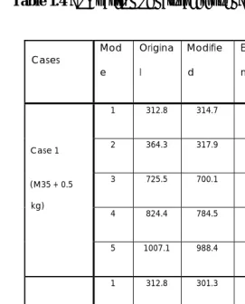
Table 1.4 Comparison of natural frequency for crankshaft system

Cases Mod

e

Origina

l

Modifie

d

Experime

nt Sensitivity

1 312.8 314.7 335 -2.84e-6

2 364.3 317.9 460 -0.001

3 725.5 700.1 750 -1.127e-6

4 824.4 784.5 805 -5.676e-6 Case 1

(M35 + 0.5

kg)

5 1007.1 988.4 1080 -3.576e-4

1 312.8 301.3 335 -0.002

2 364.3 314.7 460 -2.855e-9

3 725.5 672.5 750 -0.003

4 824.4 774.4 805 -8.246e-4 Case 2

(M1 + 1 kg)

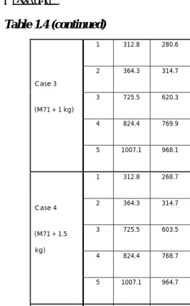
Table 1.4 (continued)

1 312.8 280.6 335 -0.004

2 364.3 314.7 460 -0.005

3 725.5 620.3 750 -0.007

4 824.4 769.9 805 -5.653e-4 Case 3

(M71 + 1 kg)

5 1007.1 968.1 1080 -0.001

1 312.8 268.7 335 -0.003

2 364.3 314.7 460 -2.018e-7

3 725.5 603.5 750 -0.004

4 824.4 768.7 805 -2.899e-4 Case 4

(M71 + 1.5

kg)

5 1007.1 964.7 1080 -8.304e-4

1 312.8 312.9 335 1.061e-7

2 364.3 364.2 460 1.600e-37

3 725.5 718.9 750 6.828e-8

4 824.4 824.5 805 7.9251e-9 Case 5

(K71+2x103_N/m

)

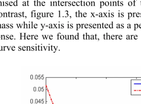
1.2.3 MASS CURVE SENSITIVITY

The intention of this chapter is to reduce vibration level of a crankshaft body by adding the least amount of mass to modify the natural frequency response. To achieve the objective, it is necessary to identify the least amount of mass and its location through sensitivity response of the body to mass variation at different location. In this example, the sensitivity to mass variation is predicted at two locations, point 35 and 71. The most effective solution is to add mass at the most sensitive location and this is optimised at the intersection points of the two-sensitivity curve. To contrast, figure 1.3, the x-axis is presented as an increment of the mass while y-axis is presented as a peak value of the frequency response. Here we found that, there are two intersection points in the curve sensitivity.

Figure 1.5 M35 and M7 sensitivity curves 567 gram

567 gram

) (gram M

Δ

∆

Hmax

567 gram 567 gram

) (gram M

Δ

∆

The first intersection point is located between 550 gram to 600 gram and the second one is located between 950 gram to 1000 gram. As, the additive mass must be predicted and could not be simply added at any location, so the result from figure 1.5 is used to decide the parameters. Here, the first intersection point (567 gram) is the best to be selected. Hence point 71 is preferred since it affects the sensitivity curve the most. However the mass sensitivity curve was decreases suddenly at peak level as the mass increases in the intersection of point mass range.

1.2.4 INVESTIGATION OF THE AMPLITUDE LEVEL

Figure 1.6 Comparison of frequency response

1.3 CONCLUSION

Partial differential sensitivity analysis method and the example using 3 degree of freedom lump’s mass and crankshaft model have been thoroughly explained in this chapter. The conclusions are drawn as follows;

The application of a modal model is good for structure modification and it is a useful technique that could be applied on a complex structure.

The accuracy of the mode shape determines the accuracy of the whole process whereby the accuracy of parameter is the key identification of allocation and quantity value for vibration reduction.

REFERENCES

1. R. B. Nelson. 1976. Simplified Calculation of Eigenvector Derivatives, AIAA, Vol. 14, No. 9: 1201-1205.

2. W. C. Mills-Curan. 1988. Calculation of Eigenvector Derivatives for Structure with Repeated Eigenvalues, AIAA, Vol. 26, No. 7: 867-871.

3. C. S. Rudisill.1974. Derivative of Eigenvalues and Eigenvectors for a General Matrix, AIAA, Vol. 12, No. 5: 721-722.

4. R. S. Fox, M. P. Kapoor. 1986. Rates of Change of Eigenvalue and Eigenvectors, AIAA, Vol. 6, No. 12: 2426-2429.

5. B. P. Wang. 1991. Improved Approximate Methods for Computing Eigenvector Derivatives, AIAA, Vol. 29, No. 6: 1018-1020,

6. H. G. Min, T. H. Tak, J. M. Lee. 1997. Kinematic Design Sensitivity Analysis of Suspension Systems using Direct Differentiation, (In Korean) Transactions of KSAE, Vol. 5, No. 1: 38-48,