Square Span Programs with Applications to Succinct NIZK Arguments

Square Span Programs

with Applications to Succinct NIZK Arguments

George Danezis1_{, C´edric Fournet}2_{, Jens Groth}1 ?_{, and Markulf Kohlweiss}2

1

University College London, UK 2

Microsoft Research

Abstract. We propose a new characterization of NP using square span programs (SSPs). We first characterize NP as affine map constraints on small vectors. We then relate this characterization to SSPs, which are similar but simpler than Quadratic Span Programs (QSPs) and Quadratic Arithmetic Programs (QAPs) since they use a single series of polynomials rather than 2 or 3.

We use SSPs to construct succinct non-interactive zero-knowledge argu-ments of knowledge. For performance, our proof system is defined over Type III bilinear groups; proofs consist of just 4 group elements, verified in just 6 pairings. Concretely, using the Pinocchio libraries, we estimate that proofs will consist of 160 bytes verified in less than 6 ms.

Keywords:Square span program, quadratic span program, SNARKs, non-interactive zero-knowledge arguments of knowledge.

1

Introduction

Gennaro, Gentry, Parno and Raykova [GGPR13] proposed a new, influential characterization of the complexity class NP using Quadratic Span Programs (QSPs), a natural extension of span programs defined by Karchmer and Wigder-son [KW93]. Their main motivation was the construction of Succinct Non-interactive Arguments of Knowledge (SNARKs). Their work has lead to fast progress towards practical verifiable computations, whereby a resource-constrained client offloads the computation of an expensive function to a computationally en-dowed server or cloud, but still intends to verify the correctness of any returned results. For instance, using Quadratic Arithmetic Programs (QAPs), a general-ization of QSPs for arithmetic circuits, Pinocchio [PHGR13] provides evidence that verified remote computation can be faster than local computation. At the same time, zero-knowledge variants of their construction enable the server to keep intermediate and additional values used in the computation private. Such constructions are at the forefront of privacy-friendly variants of Bitcoin, such as Pinocchio Coin [DFKP13] and Zerocash [BSCG+_14].

?

We introduce Square Span Programs (SSPs), a radical simplification of quadr-atic span programs, and we use them to build simpler and more efficient SNARKs and Non-Interactive Zero-Knowledge arguments (NIZKs) for the verified compu-tation of binary circuits and the verification of SAT solving, two closely related problems. Thus, SSPs can be used to build NIZK arguments to support privacy properties while guaranteeing high integrity, at a minimal cost for the verifier.

Square span programs are based on the insight that every 2-input binary gate g(a, b) =ccan be specified using (1) an affine combination`=αa+βb+γc+δ of the gate’s input and output wires that take exactly two values,`= 0 or`= 2, when the wires meet the gate’s logical specification; and (2), equivalently, as a single ‘square’ constraint (`−1)2_{= 1. Composing such constraints, a satisfying} assignment for any binary circuit (or any SAT problem) can be specified first as a set of affine map constraints, then as a constraint on the span of a set of polynomials, defining the square span program for this circuit.

Due to their conceptual simplicity, SSPs offer several advantages over previ-ous constructions for binary circuits. Their reduced number of constraints lead to smaller programs, and to lower sizes and degrees for the polynomials required to represent them, which in turn reduce the computation complexity required in proving or verifying NIZK arguments. Notably, their simpler ‘square’ form requires only a single polynomial to be evaluated for verification (instead of two for earlier QSPs, and three for Pinocchio [PHGR13]) leading to a simpler and more compact setup, smaller keys, and fewer operations required for proof and verification.

The resulting, SSP-based SNARKs may be the most compact constructions to date. For performance, our proof system is defined over Type III bilinear groups; to this end, we revisit and restate known assumptions for Type III bilin-ear groups. The communicated proofs consist of just 4 group elements (3 in the left group, and one in the right group); they can be verified in just 6 pairings, plus one multiplication for each (non-zero) bit of input, irrespective of the size of the circuit. Concretely, using the same groups as in the implementation of Pinocchio, we arrive at 160-byte proofs that we estimate can be verified in less than 6 ms, for circuits with millions of gates. For instance, our SNARKs would be entirely adequate to verify the solutions of large SAT problems offloaded to specialized servers and tools, such as those available in the annual SAT competi-tion3_{, without the need to communicate (or even reveal) their complete solutions.}

2

Square span programs

In this section we will provide new characterizations of languages in NP. First, we show that circuit satisfiability can be recast as a set of constraints on affine maps over the integers. Next, we show in Section 2.2 that this leads to the NP-completeness of square span programs as defined below. The reader may find the example in Section 2.3 useful to illustrate the transformation from circuit

3

satisfiability to square span programs. We compare square span programs to quadratic span programs in Section 2.4.

Definition 1 (Square span program). A square span program Qover the field _F consists of m+ 1polynomials v0(x), v1(x), . . . , vm(x) and a target poly-nomial t(x)such thatdeg(vi(x))≤deg(t(x))for alli= 0, . . . , m.

We say that the square span programQhas sizemand degreed= deg(t(x)). We say thatQ accepts an input (a1, . . . , a`)∈ F` if and only if there exist a`+1, . . . , am∈Fsatisfying

t(x) divides v0(x) + m

X

i=1 aivi(x)

!2

−1.

We say thatQ verifies a boolean function f : {0,1}` <sub>→ {0,1} if it accepts</sub> exactly those inputsa∈F` that satisfy a∈ {0,1}` andf(a) = 1.

In the definition, we may seef as a binary circuit or, more abstractly, as a logical specification of a satisfiability problem. In our NIZK argument system in Section 3.3 we will split the ` inputs into `u public and `w private inputs. We remark that the public ‘inputs’ are considered from the viewpoint of the verifier: for an outsourced computation for instance, they may include both the inputs sent by the clients and the outputs returned by the server performing the computation together with its proof; for a SAT problem, they may provide a partial instantiation of the problem, or a part of its solution.

This treatment is strictly more general than classic Circuit-SAT which only cares about satisfiability and thus corresponds to the special case of`u= 0, i.e., Qverifies a circuitCif it accepts exactly thosewwhereC(w) = 1. Alternatively, if we want the same SSPQto handle different circuits, it may be useful to letf be a universal circuit that takes as input an`u-bit description of a freely chosen circuitCand an`w-bit valuewand returns 1 if and only ifC(w) = 1.

2.1 The NP-completeness of affine map constraints

In this section we will show that circuit satisfiability can be recast as a set of constraints on the image of an affine mapa7→aV +b.

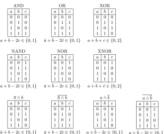
Groth, Ostrovsky and Sahai [GOS12] used that a NAND-gate with input wires a, b and output wire c can be “linearized”. Given values a, b, c ∈ {0,1}, with 0 meaning false and 1 meaning true, and writing ¯cfor 1−c, we have

c=¬(a∧b) if and only if a+b−2¯c∈ {0,1}.

AND

a b c

0 0 0

0 1 0

1 0 0

1 1 1

a+b−2c∈ {0,1}

OR

a b c

0 0 0

0 1 1

1 0 1

1 1 1

¯

a+ ¯b−2¯c∈ {0,1}

XOR

a b c

0 0 0

0 1 1

1 0 1

1 1 0

a+b+c∈ {0,2}

NAND

a b c

0 0 1

0 1 1

1 0 1

1 1 0

a+b−2¯c∈ {0,1}

NOR

a b c

0 0 1

0 1 0

1 0 0

1 1 0

¯

a+ ¯b−2c∈ {0,1}

XNOR

a b c

0 0 1

0 1 0

1 0 0

1 1 1

a+b+ ¯c∈ {0,2}

a∧b a b c

0 0 0

0 1 1

1 0 0

1 1 0

¯

a+b−2c∈ {0,1}

a∧b a b c

0 0 1

0 1 0

1 0 1

1 1 1

¯

a+b−2¯c∈ {0,1}

a∧b a b c

0 0 0

0 1 0

1 0 1

1 1 0

a+ ¯b−2c∈ {0,1}

a∧b a b c

0 0 1

0 1 1

1 0 0

1 1 1

a+ ¯b−2¯c∈ {0,1}

Table 1. Linearization of logic gates with inputsa,b and outputc. We omit the 6 remaining gates, which depend on at most one input and are not used in circuits.

Theorem 1. For any circuit C with m wires and n fan-in 2 gates for a total size ofd=m+n, there exists a matrixV ∈Zm×dand a vector b∈Zdsuch that Cis satisfiable if and only if there is a vectora∈ZmsatisfyingaV+b∈ {0,2}d. The matrixV and the vectorbcan be constructed such thataV +b∈ {0,2}d implies a∈ {0,1}m _{anda1, . . . , am corresponds to the values on the wires in a} satisfying assignment for C with the first` bits being the input wires.

Proof.We represent an assignment to the wires as a vectora∈Zm. The assign-ment is a satisfying witness for the circuit if and only if the entries belong to {0,1}, the entries respect all gates, and the output wire is 1.

It is easy to impose the conditiona∈ {0,1}m _{by requiringa(2I)∈ {0,2}}m_. (Alternatively, whenever ai ∈ {0,1} is clear from the context, for instance for the public inputsa1, . . . , a`u, this check can be omitted.)

DefineG∈_Zm×n _andδ∈

Zn such thataG+δ∈ {0,2}n corresponds to the linearization of the gates as described above, and let

V = [ 2I |G] and b= (0|δ ).

The existence ofa such that

aV +b∈ {0,2}d

is equivalent to a satisfying assignment to the wires in the circuit.

Note thatV andbas we constructed them have some additional properties. The matrixV is sparse, since it only hasm+3nnon-zero entries. The row vectors ofV andbare all linearly independent. Furthermore, all entries inV andbare small integers. The small size of the integers gives us the following corollary.

Corollary 1. For any circuitC withm wires andnfan-in 2 gates and for any p ≥8 there exist a matrix V ∈Zmp×d (with d =m+n) and a vector b ∈ Zdp (giving usm+1linearly independent row vectors) such thatCis satisfiable if and only if there exists a vectora∈Zmp satisfyingaV+b∈ {0,2}d. Furthermore, if

aV +b∈ {0,2}d _{thena∈ {0,1}}m _{andC(a1, . . . , a`) = 1.}

Relation to closest vector problem. There is an interesting connection between our construction of affine map constraints and the closest vector problem for in-teger lattices using the max-norm`∞. Consider a circuit made just from

NAND-gates; then the affine mapaV +bconstructed in the proof of Theorem 1 cannot take the value 1 for any index i = 1, . . . , d, which means the circuit is satisfi-able if and only if aV +b−1∈ {−1,0,1}d_{. This is equivalent to saying that} the lattice generated by the rows of V has a vectoraV with distance at most 1 from the target vector t = 1−b, i.e., ||aV −t||∞ ≤ 1, if and only if the

circuit is satisfiable. Our construction therefore gives a very direct reduction of the closest vector problem in integer lattices to circuit satisfiability. The NP-hardness of the closest (nearest) vector problem was first demonstrated by van Emde Boas [vEB81] but using a more complicated reduction that relied on the partition problem.

2.2 The NP-completeness of square span programs

We will now connect affine maps to square span programs, which gives a reduc-tion of square span programs to circuit satisfiability.

Corollary 1 can be reformulated to say that, for any circuit C and p ≥8, there exist V and b such that C is satisfiable if and only there exists a ∈ _Zm p satisfying

(aV +b)◦(aV +b−2) =0,

where ◦ denotes the Hadamard product (entry-wise multiplication). We can rewrite this condition as

Letr1, . . . , rd beddistinct elements ofZp for a primep≥max(d,8). Define v0(x), v1(x), . . . , vm(x) as the degree d−1 polynomials satisfying

v0(rj) =bj−1 and vi(rj) =Vi,j.

We can now reformulate Corollary 1 again. The circuitCis satisfiable if and only if there existsa∈_Zm

p such that for allrj

v0(rj) + m

X

i=1

aivi(rj)

!2

= 1.

Since the evaluations in r1, . . . , rd uniquely determine the polynomial v(x) = v0(x) +Pm

i=1aivi(x) we can rewrite the condition as

v0(x) + m

X

i=1 aivi(x)

!2

≡1 mod d

Y

j=1

(x−rj).

Theorem 2. A circuitC with mwires and nfan-in 2 gates has for any prime p≥max(n,8)a square span program of sizemand degreed=m+nthat verifies it overZp.

Proof. From the discussion above, we see that for any circuit C with m wires and n gates there exists polynomials v0(x), v1(x), . . . , vm(x) and distinct roots r1, . . . , rdsuch that Cis satisfiable if and only if

d

Y

j=1

(x−rj) divides v0(x) + m

X

i=1 aivi(x)

!2

−1.

Define t(x) = Qd

j=1(x−rj) to get an SSP Q = v0(x), v1(x), . . . , vm(x), t(x)

that verifiesC over_Zp.

2.3 Example

As a small example of the process of generating a square span program, consider a circuit consisting of a single XOR-gate a3 =a1⊕a2 (here ` = `u+`w = 2 with `u= 0 and `w = 2). To guaranteea1, a2, a3∈ {0,1} and the XOR-gate is respected we use the constraints 2ai∈ {0,2}anda1+a2+a3∈ {0,2}. The output should be a3= 1, which we represent with the constraint 3¯a3 = 3(1−a3) = 0. We add the latter constraint to the output wire’s equation to get the combined a1+a2−2a3+ 3∈ {0,2}, which at the same time guaranteesa3=a1⊕a2 and a3= 1. We can represent the constraints as

aV +b= (a1, a2, a3)





2 0 0 1

0 2 0 1

0 0 2 −2



+ (0,0,0,3) ∈ {0,2}

The satisfiability of the circuit can therefore be represented by 4 quadratic equa-tions

(2a1−1)2= 1 (2a2−1)2= 1 (2a3−1)2= 1 (a1+a2−2a3+ 2)2= 1 corresponding to (aV +b−1)◦(aV +b−1) =1.

To get a square span program, letp≥8 be a prime andr1, r2, r3, r4be four distinct elements inZp. Pick degree 3 polynomialsv0(x), v1(x), v2(x), v3(x) such that

v0(r1), v0(r2), v0(r3), v0(r4)=b−1 = (−1,−1,−1,2)

and





v1(r1) v1(r2) v1(r3) v1(r4) v2(r1) v2(r2) v2(r3) v2(r4) v3(r1) v3(r2) v3(r3) v3(r4)



=V = 



2 0 0 1

0 2 0 1

0 0 2 −2



.

Let t(x) = (x−r1)(x−r2)(x−r3)(x−r4) to get a square span program v0(x), v1(x), v2(x), v3(x), t(x)

for the circuit such that

t(x) divides v0(x) +a1v1(x) +a2v2(x) +a3v3(x) 2

−1

if and only ifa1, a2, a3 satisfy the circuit, i.e.,a1, a2 ∈ {0,1}, a3 = 1 anda3= a1⊕a2.

2.4 Comparison to quadratic span programs

Square span programs can be seen as a simplification of quadratic span programs. Below we recall the definition of quadratic span programs given by Gennaro, Gentry, Parno and Raykova [GGPR13].

Definition 2. A quadratic span program over a field F contains two sets of polynomials V ={v0₀(x), . . . , vm(x)} andW ={w0₀(x), . . . , wm(x)} and a target polynomial t(x). It also contains a partition of the indices I ={1, . . . , m} into I =Ilabeled∪ Ifree and a further partitionIlabeled=∪

`,1

i=1,j=0Ii,j. For input4 _{y ∈ {0,1}}`_{, let I}

y = Ifree∪`i=1Ii,yi be the set of indices that “belong” to y. The quadratic span programaccepts an inputy ∈ {0,1}` _{if and} only if there existai, bi∈F such that

t(x) divides



v00(x) +

X

i∈Iy aivi(x)



· 

w00(x) +

X

i∈Iy

biwi(x)



.

We say the quadratic span program verifies a boolean functionf :{0,1}`_→ {0,1} if it accepts exactly those inputs y wheref(y) = 1. We say the size of the quadratic span program ism and the degree isdeg(t(x)).

4

Size and degree of Span Programs

Size Degree

Quadratic span programs [GGPR13] 36n 130n

Quadratic span programs (Lipmaa) [Lip13] 14n−14`−2 11n−12`−2

Square span programs m m+n−`u

Table 2.Costs compared with prior work (`input wires, out of which`u are public,

mwires in total and ngates). In a circuit with fan-in 2 gatesm≤2n+ 1, so we get rough bounds of size 2nand degree 3nwhen computed as a function of the number of gatesnonly (ignoring`u).

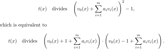
A square span program uses the simpler condition

t(x) divides v0(x) + m

X

i=1 aivi(x)

!2

−1,

which is equivalent to

t(x) divides v0(x) + 1 + m

X

i=1 aivi(x)

!

· v0(x)−1 + m

X

i=1 aivi(x)

!

.

A square span program can therefore be seen as a particularly simple type of quadratic span program where w0₀(x) = v0₀(x)−2 and wi(x) = vi(x) and ai =bi. Furthermore, Ilabeled ={1, . . . , `} with Ii,yi ={i} and Ii,¯yi =∅, and Ifree={`+ 1, . . . , m}.

The compilation of a circuit into a quadratic span programs in [GGPR13] has a significant overhead. For a circuit with`input wires andmwires in total and ngates, the size of the resulting quadratic span program is 36nand the degree is 130n. Lipmaa [Lip13] gave a class of more efficient quadratic span programs. Included in this class is a quadratic span program of size 14n−14`−2 and degree 11n−12`−2. In comparison with these works our (square) quadratic span programs are much more compact with size m−`u and degree m+n− `u (assuming the verifier checks its inputs are all in {0,1}.) These costs are summarised in Table 2.

A further advantage compared to the previous works is that we consider all types of logic gates, whereas they only consider NAND, AND and OR gates. We would expect that their constructions can be generalized to handle other logic gates but do not know whether this would increase the cost.

3

Succinct non-interactive arguments of knowledge

We will now use square span programs to construct succinct non-interactive zero-knowledge arguments of knowledge using bilinear groups.

Notation. Given two functions f, g : N → [0,1] we write f(λ) ≈ g(λ) when |f(λ)−g(λ)|=λ−ω(1). We say thatf is negligiblewhenf(λ)≈0 and thatf is overwhelmingwhenf(λ)≈1.

We writey =A(x;r) when the algorithm A on input xand randomness r, outputsy. We writey←A(x) for the process of picking randomnessrat random and settingy =A(x;r). We also writey←Sfor samplingyuniformly at random from the setS. We will assume it is possible to sample uniformly at random from sets such asZp.

Following Abe and Fehr [AF07] we write (y;z)← (A k XA)(x) when Aon

inputxoutputsyandXAon the same input (including random coins) outputsz.

3.1 Non-interactive zero-knowledge arguments of knowledge

Let{Rλ}λ∈Nbe a sequence of families of efficiently decidable binary relationsR.

For pairs (u, w)∈Rwe calluthe statement andwthe witness. A non-interactive argument for{Rλ}λ∈N is a quadruple of efficient algorithms (Setup,Prove,Vfy,

Sim) working as follows:

(σ, τ)←Setup(1λ_{, R): the setup algorithm takes as input a security parameterλ} and a relation R ∈ Rλ and returns a common reference string σ and a simulation trapdoorτ for the relationR.

π←Prove(σ, u, w): the prover algorithm takes as input a common reference stringσfor a relationR and (u, w)∈Rand returns an argument π. 0/1←Vfy(σ, u, π): the verification algorithm takes as input a common reference

string, a statementuand an argumentπand returns 0 (reject) or 1 (accept). π←Sim(τ, u): the simulator takes as input a simulation trapdoor and a

state-mentuand returns an argumentπ.

Definition 3. We say(Setup,Prove,Vfy,Sim)is a perfect non-interactive zero-knowledge argument of zero-knowledge for {Rλ}λ∈N if it has perfect completeness,

perfect zero-knowledge and computational knowledge soundness as defined below.

Perfect completeness. Completeness says that, given any true statement,

an honest prover should be able to convince an honest verifier. For all λ∈ _N, R∈ Rλ, (u, w)∈R

Prh(σ, τ)←Setup(1λ, R);π←Prove(σ, u, w) : Vfy(σ, u, π) = 1i= 1.

Perfect zero-knowledge.An argument is zero-knowledge if it does not leak

Sim) is perfect zero-knowledge if for all λ ∈ _N, R ∈ Rλ,(u, w) ∈ R and all adversariesA, we have

Prh(σ, τ)←Setup(1λ, R);π←Prove(σ, u, w) :A(σ, τ, π) = 1i = Prh(σ, τ)←Setup(1λ, R);π←Sim(τ, u) :A(σ, τ, π) = 1i.

Computational knowledge soundness.We call (Setup,Prove,Vfy,Sim) an

argument of knowledge if there is an extractor that can compute a witness when-ever the adversary produces a valid argument. The extractor gets full access to the adversary’s state, including any random coins.

Formally, we require that, for all sequences (Rλ)λ∈Nof polynomially bounded

relations in {Rλ}λ∈N and non-uniform polynomial time adversaries A, there

exists a non-uniform polynomial time extractorXA such that

Pr

(σ, τ)←Setup(1λ, Rλ) ((u, π);w)←(A k XA)(σ) :

(u, w)∈/Rλ Vfy(σ, u, π) = 1

≈0.

Remark. Our notion of knowledge soundness guarantees security against an adaptive adversary, cf. [AF07], that chooses the instance u depending on the CRS σ. However, to get adaptive security for circuit satisfiability, Rλ has to be universal, i.e., it has to check that a circuituis satisfiable. For performance reasons, this is usually not what one wants, and adaptive soundness for a more restrictive Rλ is preferable. See Lipmaa [Lip14] for how to achieve adaptive soundness for some NP-complete languages, not including circuit satisfiability, while avoiding universal circuits.

3.2 Bilinear groups

Let G be a bilinear group generator that, on security parameter λ, returns (p,_G,_Gˆ,_GT, e)← G(1λ) with the following properties:

– _G,_Gˆ,_GT are groups of prime orderp;

– e:_G×Gˆ →GT is a bilinear map, that is, for all U ∈G, V ∈Gˆ, a, b∈Z, we havee(Ua_{, V}b_{) =e(U, V)}ab_;

– ifGis a generator forGand ˆGis a generator for ˆGthene(G,Gˆ) is a generator forGT; and

– there are efficient algorithms for computing group operations, evaluating the bilinear map, deciding membership of the groups, deciding equality of group elements and sampling generators of the groups.

The q-power knowledge of exponent assumption.The knowledge of

ex-ponent assumption (KEA) introduced by Damg˚ard [Dam91] says that given G, G0 =Gα_{it is infeasible to createV, V}0 _{such thatV}0 _=Vα_{without knowinga} such thatV =Ga_andV0_=G0a

. Bellare and Palacio [BP04] extended this to the KEA3 assumption, which says that givenG, Gs_{, G}0_{, G}0s

it is infeasible to create V, V0 =Vα _{without knowinga0, a1 such thatV =G}a0_(Gs₎a1_{. This assumption}

has been used also in symmetric bilinear groups by Abe and Fehr [AF07] who called it the extended knowledge of exponent assumption.

Theq-power knowledge of exponent assumption is a generalization of these assumptions in bilinear groups. It says that given (G,G, Gˆ s_,Gˆs_{, . . . , G}sq_,Gˆsq₎ it is infeasible to create V,Vˆ such that e(V,Gˆ) = e(G,Vˆ) without knowing a0, . . . , aq such thatV =Q

q i=0(G

si

)ai_{. Theq-power knowledge of exponent} as-sumption was introduced in [Gro10] for symmetric bilinear groups using ˆG=Gα withαchosen at random. Here we adapt it with minor modifications to the gen-eral setting where it may be the case that _G6= ˆ_GandG,Gˆ belong to different groups.

Definition 4 (q-PKE). The q(λ)-power knowledge of exponent assumption holds relative toGfor the classZof auxiliary input generators if, for every non-uniform polynomial time auxiliary input generatorZ ∈ Zand non-uniform poly-nomial time adversary A, there exists a non-uniform polynomial time extrac-torXA such that

Pr



   

gk:= (p,G,Gˆ,GT, e)← G(1λ);G←G∗ s←Z∗p;z←Z(gk, G, . . . , Gs

q

); ˆG←Gˆ∗ (V,Vˆ;a0, . . . , aq)←(A k XA)(gk, G,G, . . . , Gˆ s

q

,Gˆsq, z) : e(V,Gˆ) =e(G,Vˆ) ∧ V 6=GPqi=0aisi



   

≈ 0.

An adaptation of the proof in Groth [Gro10] shows that theq-PKE assumption holds in the generic bilinear group model.

As demonstrated by Bitansky, Canetti, Paneth and Rosen [BCPR13], if in-distinguishability obfuscators [BGI+_12,GGH+_{13] exist, then there are auxiliary} input generators for which theq-PKE assumption does not hold. However, their counterexample is specifically tailored to make extraction difficult and, as they explain, theq-PKE assumption may hold for “benign” auxiliary input genera-tors. We will later use auxiliary input generators that generate group elements in G and ˆG in a specific manner according to the relations Rλ and we will conjecture that such auxiliary input generators are benign and that the q-PKE assumption holds with respect to them.

The q-power Diffie-Hellman assumption.Theq-power Diffie-Hellman

Definition 5 (q-PDH). The q(λ)-power Diffie-Hellman assumption holds rel-ative toG if for all non-uniform probabilistic polynomial time adversaries A

Pr



 

gk:= (p,_G,_Gˆ,_GT, e)← G(1λ);G←G∗; ˆG←Gˆ∗;s←Z∗p Y ← A(gk, G,G, . . . , Gˆ sq_,Gˆsq_{, G}sq+2_,Gˆsq+2_{, . . . , G}s2q_,Gˆs2q_{) :} Y =Gsq+1





 ≈ 0.

An adaptation of the proof in Groth [Gro10] shows that theq-PDH assumption holds in the generic bilinear group model.

The q-target group strong Diffie-Hellman assumption.We adapt the

strong Diffie-Hellman assumption [BB08] in the target group [PHGR13] to the asymmetric setting. It says that given (G,G, . . . , Gˆ sq,Gˆsq) it is hard to find an r∈Zp and computee(G,Gˆ)

1

s−r.

Definition 6 (q-TSDH).Theq(λ)-target group strong Diffie-Hellman assump-tion holds relative toG if for all non-uniform probabilistic polynomial time ad-versariesA

Pr



 

(p,G,Gˆ,GT, e)← G(1λ);G←G∗; ˆG←Gˆ∗;s←Z∗p (r, Y)← A(p,G,Gˆ,GT, e, G,G, . . . , Gˆ s

q ,Gˆsq) : r∈_Zp\ {s} ∧ Y =e(G,Gˆ)

1

s−r





 ≈ 0.

An adaptation of the proof in Boneh and Boyen [BB08] shows that theq-TSDH assumption holds in the generic bilinear group model.

3.3 Succinct perfect NIZK arguments

We will now construct succinct and perfect NIZK arguments of knowledge for any functions `u, `w and families{R}λ of relationsR of pairs (u, w)∈ {0,1}`u(λ)× {0,1}`w(λ) _{that can be computed by polynomial size circuits with m(λ) wires} andn(λ) gates for a total size ofd(λ) =m(λ) +n(λ).

(σ, τ)←Setup(1λ, R): Rungk:= (p,G,Gˆ,GT, e)← G(1λ). ParseRas a boolean circuitCR : {0,1}`u<sub>× {0,1}</sub>`w _{→ {0,1}. Generate a square span program} Q = v0(x), . . . , vm(x), t(x)

that verifies CR over Zp. Pick G ← G∗ and ˆ

G,G˜ ←Gˆ∗andβ, s←Z∗psuch that t(s)6= 0. Return

σ = (gk, G,G, . . . , Gˆ sd,Gˆsd,{Gβvi(s)}i>`u, G

βt(s)_{,G,˜ G˜}β_{, Q)} τ = (σ, β, s).

π←Prove(σ, u, w): Parse uas (a1, . . . , a`u) ∈ {0,1}`u and use w to compute a`_u+1, . . . , amsuch thatt(x) dividesv0(x) +Pm

i=1aivi(x)

2

−1. Pickδ←Zp and let

h(x) = (v0(x) +

Pm

i=1aivi(x) +δt(x)) 2

−1

Use linear combinations of the elements inσto compute

H =Gh(s) Vw=G

Pm

i>`uaivi(s)+δt(s) Bw=Gβ(Pmi>`uaivi(s)+δt(s)) _Vˆ _{= ˆG}v0(s)+Pmi=1aivi(s)+δt(s)

and returnπ= (H, Vw, Bw,Vˆ).

0/1←Vfy(σ, u, π): Parseuas (a1, . . . , a`u)∈ {0,1}`uandπas (H, Vw, Bw,Vˆ)∈ G3×Gˆ. ComputeV =Gv0(s)+P`ui=1aivi(s)_V

wand return 1 if and only if e(V,Gˆ) =e(G,Vˆ) e(H,Gˆt(s)) =e(V,Vˆ)e(G,Gˆ)−1 e(Vw,G˜β) =e(Bw,G˜). π←Sim(τ, u): Parseuas (a1, . . . , a`<sub>u</sub>)∈ {0,1}`u _{and pickδw←}

Zpat random. Let

h=

v0(s) +P `u

i=1aivi(s) +δw

2

−1

t(s)

and returnπ= (Gh, Gδw_{, G}βδw_,Gˆv0(s)+P`ui=1aivi(s)+δw_).

LetZbe a family of non-uniform polynomial time auxiliary input generators Z such that each of them corresponds to sequences of relations (Rλ)λ∈Nin a family

of relations {Rλ}λ∈N. They work such thatZ corresponding to (Rλ)λ∈Non

in-put (p,G,Gˆ,GT, e, G, . . . , Gs q

) generates the final part of the common reference string, i.e., returns z= ({Gβvi(s)_}

i>`u, G

βt(s)_,G,˜ _G˜β_{, Q).}

Theorem 3. The construction above is a perfect NIZK argument for the family of relations {Rλ}λ∈Nbounded by d(λ) with computational knowledge soundness

if the d(λ)-PKE, d(λ)-PDH and d(λ)-SDH assumptions hold relative to G and the family of auxiliary input generator Z defined above.

Proof.Perfect completeness follows by direct verification.

Perfect zero-knowledge follows from observing that both a real argument and a simulated argument have a uniformly random Vw because t(s)6= 0 and δ, δw are chosen uniformly at random. OnceVw has been fixed, the verification equations uniquely determineBw,Vˆ andH. This means that for any (u, w)∈R both the real arguments and the simulated arguments are chosen uniformly at random such that the verification equations will be satisfied.

We now describe the witness-extractor for computational knowledge sound-ness. The setup algorithm first generates a bilinear group (p,_G,_Gˆ,_GT, e) ← G(1λ_{) and picksG ←}

G∗ and s←Z∗p, which are used to compute G, . . . , Gs d

. This is exactly like the input given to the auxiliary input generator in a d -PKE challenge. The setup algorithm now generates a square span program Q over_Zp for the relationRλ and elements{Gβvi(s)}i>`u and ˜G,G˜β. We can con-sider this as part of the auxiliary inputz that Z outputs in the d-PKE defini-tion. More precisely, let A0 _{be the d-PKE adversary that, on (p,}

G,Gˆ,GT, e, G,G, . . . , Gˆ sd,Gˆsd) and auxiliary input z = ({Gβvi(s)_}

i>`u, G

V =Gv0(s)+P`ui=1aivi(s)Vwwhenu= (a1, . . . , a`

u)∈ {0,1}

`u_{. LetX}

A0 be the

cor-responding extractor according to thed-PKE assumption that returnsc0, . . . , cd such that V = GPdi=0cisi _{when e(V,G}ˆ_{) = e(G,V}ˆ_{). Our witness-extractor X}

A

givenσruns (V,Vˆ;c0, . . . , cd)←(A0_{k X}

A0)(p,_G,_Gˆ,_GT, e, G,G, . . . , Gˆ s

d

,Gˆsd_{, z),} which defines a polynomialPd

i=0cix

i_{. Defineδ=cd to get a degreed−1} poly-nomialv(x) =Pd

i=0cix

i_{−δt(x). If it is possible to write the polynomial on the} formv(x) =v0(x) +Pm

i=1aivi(x) such that (a1, . . . , am)∈ {0,1}

m_{is a satisfying} assignment for the circuitCR withu= (a1, . . . , a`u) then the extractor returns w= (a`u+1, . . . , a`u+`w).

We will now show that with all but negligible probability the extracted polynomial v(x) does indeed provide a valid witness w ∈ {0,1}`w _{such that} (u, w) ∈ Rλ. Let Qbe the square span program (v0(x), . . . , vm(x), t(x)) speci-fied in σ that verifies Rλ overZp. We know by Theorem 2 that if t(x) divides v(x)2−1 andvmid(x) =Pd

i=0cix

i_−v0(x)−P`u

i=1aivi(x) belongs to the span of {vi(x)}i>`u then indeedw∈ {0,1}

`w_{and (u, w)∈ R}

λ. So we will in the following show that the two cases,t(x) does not dividev(x)2−1 orvmid(x) is not in the appropriate span both happen with negligible probability breaking thed-TSDH assumption or thed-PDH assumption respectively.

Given ad-TSDH challenge (p,G,Gˆ,GT, e, G,G, . . . , Gˆ s d

,Gˆsd_{), we pick β ←} Z∗p and roots r1, . . . , rd in the same way the setup algorithm does and simulate a common reference string σ. Suppose the adversary and extractor return u= (a1, . . . , a`<sub>u</sub>) ∈ {0,1}`u_{, a valid proof π = (H, Vw, Bw,V}ˆ_{) and c0, . . . , cd such} that V =Gv0(s)+P`ui=1aivi(s)_Vw=GPdi=0cisi_{. Letv(x) =}Pd

i=0cix

i_{−δt(x) with} δ=cd as before and definep(x) = (v(x) +δt(x))2−1 and supposep(x) is not divisible byt(x). Letri be a root of t(x) such thatx−ri does not dividep(x). We can writep(x) =a(x)(x−ri) +b, wherea(x) is a degree 2d−1 polynomial in Zp[x] and b ∈ Z∗p. The verification equatione(H,Gˆ

t(s)_{) =e(V,Vˆ)e(G,Gˆ)}−1 gives us e(H,Gˆst−(s_ri)_{) = e(G,G}ˆ₎a(s)+s−b_{ri. The adversary can use generic group}

operations on the d-TSDH challenge to compute ˆG t(s)

s−ri _ande(G,Gˆ₎a(s)_{, which} allows it to deduce e(G,Gˆ)s−bri_{. Rasing this to the power b}−1 _{gives a solution} (ri, e(G,Gˆ)s−1ri_{) to thed-TSDH challenge.}

Given ad-PDH challenge (p,_G,_Gˆ,_GT, e, G,G, . . . , Gˆ s d

,Gˆsd_{, G}sd+2_,Gˆsd+2_{, . . . ,} Gs2d,Gˆs2d) we pick a random degreedpolynomiala(x) such thata(x)vi(x) has coefficient 0 for xd _{for all `}

u < i ≤ m and a(x)t(x) also has coefficient 0 for xd_{. There are d+`}

u−m−1 > 0 degrees of freedom in choosing a(x) so for a polynomial vmid(x) outside the span of {vi(x)}mi=`u and t(x) the polynomial a(x)vmid(x) has a random coefficient for xd.

common reference string

σ= (p,G,Gˆ,GT, e, G,G, . . . , Gˆ s d

,Gˆsd,{Gβvi(s)}i>`u, G

βt(s)_{,G,˜ G˜}β_{, Q).} Suppose the adversary and extractor returnu= (a1, . . . , a`u)∈ {0,1}`u, a valid proofπ= (H, Vw, Bw,Vˆ) andc0, . . . , cd such thatV =G

P

i=0cisi_{. Define} vmid(x) =P

d

i=0cixi−v0(x)−P `u

i=1aivi(x). Due to the random choice ofbthe valueβ(s) =a(s)s+bdoes not reveal anything abouta(x), so ifvmid(x) is outside the span of{vi(x)}i>`u andt(x) then a(x)vmid(x) has a random coefficient for xd+1_{. With probability 1−}1

p this means the adversary returnsBw=Gβ(s)vmid(s) whereβ(x)vmid(x) =P2d

i=0bix

i _{is a known polynomial with a non-trivial} coeffi-cientbd+16= 0 forxd+1. We can now take an appropriate linear combination of Bwand the elementsG, . . . , Gsd, Gsd+2, . . . , Gs2dto computeGsd+1, which solves

thed-PDH challenge.

The proof of Theorem 3 suffers a computational overhead in the reduction by using an extractor XA for A. Except for this computational overhead, the

security reduction for knowledge soundness is tight. It is possible to eliminate theq-TSDH assumption and rely solely on theq-PKE andq-PDH assumptions, but then the security reduction loses a factorqand is therefore not tight.

3.4 Efficiency

In this section, we will assume our NIZK argument is instantiated with the square span program that we constructed in Section 2.2. This choice of square span program enables a number of optimizations that makes the argument highly efficient.

The prover has to compute

Vw = GPmi>`uaivi(s)+δt(s) Bw = Gβ(Pmi>`uaivi(s)+δt(s))

ˆ

V = Gˆv0(s)+Pmi=1aivi(s)+δt(s)_. It is possible to compute the polynomials Pm

i>`uaivi(x) +δt(x) and v0(x) +

Pm

i=1aivi(x) +δt(x) and then compute the appropriate exponentiations of the polynomials evaluated insusing the elementsG, ˆG,. . . , Gsd_{, ˆG}sd_,{Gβvi(s)_}

i>`u, andGβt(s)_{from the common reference string. However, this requiresO(d)} expo-nentations to the coefficients of the polynomials. Following [GGPR13] a signifi-cant saving can be made by precomputing{Gvi(s)_}

i>`u,G

t(s) _and{Gˆvi(s)_}m i=0, ˆ

Gt(s)_{. Since eacha}

i∈ {0,1}this makes it possible to computeVw, Bwand ˆV us-ing at most 3m+ 1−2`u multiplications and 3 exponentiations. (Pragmatically, taking advantage of our uniform support for all gates, we can profile the SSP and ‘flip’ internal values fromai toaito ensure thatai is more often equal to 0 than to 1, thereby on average performing less than half of those multiplications.)

The prover also has to computeH =Gh(s)_{, whereh(x) =} (v(x)+δt(x))2−1 t(x) with v(x) =v0(x) +Pm

i=1aivi(x) and t(x) =

Qd

dpointsr₁0, . . . , r0_d using two discrete Fourier transforms as follows. The degree d−1 polynomial v(x) is uniquely determined by its evaluation in the dpoints r1, . . . , rd. In our square span program the evaluations in the pointsr1, . . . , rdcan be computed easily given the values of the wires in the circuit. Using an inverse discrete Fourier transform, we compute the coefficients of v(x) = Pd−1

i=0 cix i_. Let γ ∈Z∗p be given such that r01, . . . , rd0 defined as ri0 = γiri gives us 2d dis-tinct valuesr1, . . . , rd, r01, . . . , rd0. Computec0i=γ

i_{ci to get the coefficients of the} polynomial v0(x) =Pd−1

i=0 c

0

ixi and use a discrete Fourier transform to evaluate v0(x) in r1, . . . , rd. This gives us evaluations of v(x) in the points r₁0, . . . , r0_d since v(r0_j) = v0(rj). We have h(x) =

v(x)2₋₁

t(x) + 2δv(x) +δ

2_{t(x). Assuming} t(r₁0)−1, . . . , t(r0_d)−1 have been precomputed, it only costs 3dmultiplications in Zp to evaluate v(x)

2₋₁

t(x) + 2δv(x) in thedpointsr

0

1, . . . , r0d. Using Lagrange inter-polation in the exponent, this allows us to compute

Gv(st)2−1(s) +2δv(s)₌

d

Y

j=1 (G`0j(s)₎

v(r0_j)2−1

t(r_j0) +2δv(r 0

j)

where`0_j(x) is the Lagrange basis polynomial forr0_j. By multiplying with (Gt(s)₎δ2 we then getGh(s).

To speed up the computation, we can set up a modified common reference string for the prover

σProve=

p,G,Gˆ,GT, e, G,G,ˆ {Gvi(s)}i>`u,{Gˆ vi(s)_}

i>`u,{G βvi(s)_}

i>`u, Gβt(s),G,˜ G˜β, γ,{t(r0_j)−1}d

j=1,{G `0_j(s)_}d

j=1, G t(s)_{, Q}

!

.

The computational cost for the prover is dominated byd exponentations in_G and 2 discrete Fourier transforms in _Zp. The two discrete Fourier transforms costO(dlog2d) multiplications in general but the computation can be reduced to O(dlogd) multiplications when Zp is of a form amenable to using the fast Fourier transform.

The verifier needs to computeV =Gv0(s)+Pi`u=1aivi(s)_{Vw and evaluate three} pairing product equations e(V,Gˆ) = e(G,Vˆ), e(H,Gˆt(s)) = e(V,Vˆ)e(G,Gˆ)−1, ande(Vw,G˜β) =e(Bw,G˜).The verifier does not need the full common reference string but can use a more compact common reference string

σVfy=

p,_G,_Gˆ,_GT, e, G,{Gvi(s)}`ui=0,G,ˆ Gˆ

t(s)_{,G,˜ G˜}β_,

which only has`u+ 6 group elements.5 <sub>Verification is also computationally</sub> effi-cient, in the worst case it requires`u+ 1 multiplications inG, one multiplication in GT and 6 pairings if we precomputee(G,Gˆ)−1.

For a large circuit, the cost of verification can be much smaller than the cost of evaluating the circuit itself, even if the witnesswis known to the verifier. This

5

Using the binary representation of the public inputufrom [PHGR13] this can be further reduced tod`u

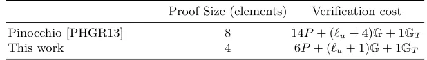
Proof size and verification cost comparison with Pinocchio

Proof Size (elements) Verification cost

Pinocchio [PHGR13] 8 14P+ (`u+ 4)G+ 1GT

This work 4 6P+ (`u+ 1)G+ 1GT

Table 3.Size in number of group elements (eitherG or ˆG), performance in terms of

pairings (P) or multiplications inG orGT respectively.

makes the NIZK argument a succinct non-interactive argument of knowledge that is suitable for verifiable computation protocols.6

Partly due to the lack of benchmarks, it is hard to compare the performance of SNARK protocols quantitatively without carefully reimplementing them. Table 3 compares the proof sizes and operations performed by the verifier between our protocol and Pinocchio, arguably the state of the art in terms of proof size and verification speed for QAPs. On this basis and the numbers reported in [PHGR13], we conservatively estimate that an SSP implementation based on the Pinocchio library would offer 160-byte proofs verified in less than 6 ms.

4

Conclusion

We introduce a representation of logic circuits, or predicates on propositional formulae, using quadratic constraints on an affine map. The map is built using a linearization of each gate, and a set of constraints to ensure all values of wires are binary. This leads to a simple and elegant formulation of square span programs, and in turn to efficient, minimalistic constructions for NIZKs and SNARKs.

The simplifications are twofold: (i) our representation of boolean functions no longer requires wire checkers and (ii) square span programs consist of only a single set of polynomials that are summed and squared. The former improves prover efficiency, while the key advantage of the latter are SNARKs with an extremely compact proof, consisting of only four group elements, and an efficient verification procedure compared to more generic QSP characterisations of the same program.

As can be expected, binary programs such as SSPs remain less efficient than arithmetic programs for verifying computations on integers, involving e.g. 32-bit additions and multiplications. Those operations have to be encoded as binary adders and multipliers, leading to a significant blow-up in circuit size and com-putation costs for the prover. It remains an open problem how to extend the SSP approach with ideas from QAPs to verify such computations without sacrificing its conceptual simplicity and short proofs.

6 _{In some cases, for instance when outsourcing computation, the verifier may be the}

one that sets up the common reference string. In that case the verifier may knowβ

References

[AF07] Masayuki Abe and Serge Fehr. Perfect NIZK with adaptive soundness. In

TCC, volume 4392 ofLecture Notes in Computer Science, pages 118–136, 2007.

[BB08] Dan Boneh and Xavier Boyen. Short signatures without random ora-cles and the sdh assumption in bilinear groups. Journal of Cryptology, 21(2):149–177, 2008.

[BCPR13] Nir Bitansky, Ran Canetti, Omer Paneth, and Alon Rosen. Indistinguisha-bility obfuscation vs. auxiliary-input extractable functions: One must fall. IACR Cryptology ePrint Archive, Report 2013/641, 2013.

[BGI+12] Boaz Barak, Oded Goldreich, Russell Impagliazzo, Steven Rudich, Amit Sahai, Salil P. Vadhan, and Ke Yang. On the (im)possibility of obfuscating programs. Journal of the ACM, 59(2):6, 2012.

[BP04] Mihir Bellare and Adriana Palacio. Towards plaintext-aware public-key en-cryption without random oracles. InASIACRYPT, volume 3329 ofLecture Notes in Computer Science, pages 48–62, 2004.

[BSCG+_{14] Eli Ben-Sasson, Alessandro Chiesa, Christina Garman, Matthew Green,} Ian Miers, Eran Tromer, and Madars Virza. Zerocash: Practical decen-tralized anonymous e-cash from bitcoin. InProceedings of the 2014 IEEE Symposium on Security and Privacy. IEEE, May 2014.

[Dam91] Ivan Damg˚ard. Towards practical public key systems secure against chosen ciphertext attacks. InCRYPTO, volume 576 ofLecture Notes in Computer Science, pages 445–456, 1991.

[DFKP13] George Danezis, C´edric Fournet, Markulf Kohlweiss, and Bryan Parno. Pinocchio coin: building zerocoin from a succinct pairing-based proof sys-tem. In Martin Franz, Andreas Holzer, Rupak Majumdar, Bryan Parno, and Helmut Veith, editors,PETShop@CCS, pages 27–30. ACM, 2013. [GGH+13] Sanjam Garg, Craig Gentry, Shai Halevi, Mariana Raykova, Amit Sahai,

and Brent Waters. Candidate indistinguishability obfuscation and func-tional encryption for all circuits. InFOCS, pages 40–49, 2013.

[GGPR13] Rosario Gennaro, Craig Gentry, Bryan Parno, and Mariana Raykova. Quadratic span programs and succinct nizks without pcps. In EURO-CRYPT, volume 7881 ofLecture Notes in Computer Science, pages 626– 645, 2013.

[GOS12] Jens Groth, Rafail Ostrovsky, and Amit Sahai. New techniques for nonin-teractive zero-knowledge. Journal of the ACM, 59(3):11:1–11:35, 2012. [GPS08] Steven D. Galbraith, Kenneth G. Paterson, and Nigel P. Smart. Pairings for

cryptographers. Discrete Applied Mathematics, 156(16):3113–3121, 2008. [Gro10] Jens Groth. Short pairing-based non-interactive zero-knowledge

argu-ments. InASIACRYPT, volume 6477 ofLecture Notes in Computer Sci-ence, pages 321–340, 2010.

[KW93] M. Karchmer and A. Wigderson. On span programs. InIn Proc. of the 8th IEEE Structure in Complexity Theory, pages 102–111. IEEE Computer Society Press, 1993.

[Lip13] Helger Lipmaa. Succinct non-interactive zero knowledge arguments from span programs and linear error-correcting codes. InASIACRYPT, volume 8269 ofLecture Notes in Computer Science, pages 41–60, 2013.

[PHGR13] Bryan Parno, Jon Howell, Craig Gentry, and Mariana Raykova. Pinocchio: Nearly practical verifiable computation. InIEEE Symposium on Security and Privacy, pages 238–252, 2013.

[Val76] Leslie G. Valiant. Universal circuits (preliminary report). InSTOC, pages 196–203, 1976.