Fast Evaluation of Polynomials over Binary
Finite Fields and Application to Side-channel
Countermeasures
?Jean-S´ebastien Coron1, Arnab Roy1,2, Srinivas Vivek1 1
University of Luxembourg
{jean-sebastien.coron, srinivasvivek.venkatesh}@uni.lu
2
Technical University of Denmark
Abstract. We describe a new technique for evaluating polynomials over binary finite fields. This is useful in the context of anti-DPA counter-measures when an S-box is expressed as a polynomial over a binary finite field. Forn-bit S-boxes our new technique has heuristic complexity
O(2n/2/√n) instead ofO(2n/2) proven complexity for the Parity-Split method. We also prove a lower bound ofΩ(2n/2/√n) on the complexity of any method to evaluaten-bit S-boxes; this shows that our method is asymptotically optimal. Here, complexity refers to the number of non-linear multiplications required to evaluate the polynomial corresponding to an S-box.
In practice we can evaluate any 8-bit S-box in 10 non-linear multiplica-tions instead of 16 in the Roy-Vivek paper from CHES 2013, and the DES S-boxes in 4 non-linear multiplications instead of 7. We also eval-uate any 4-bit S-box in 2 non-linear multiplications instead of 3. Hence our method achieves optimal complexity for the PRESENT S-box.
1
Introduction
The implementations of cryptographic algorithms on devices like PCs, micro-controllers, smart cards, etc. leak secret information to an adversary. Typical examples of such leakages are electro-magnetic emissions, power consumption and even acoustic emanations. An adversary can use this information to recover the secret key by applying different statistical techniques. Differential Power Analysis (DPA) – the most widely known and powerful technique – is based on statistical analysis of the power consumption of a device [KJJ99]. Other tech-niques including Template Attacks, Correlation Power Analysis Attacks (CPA), etc. were proposed in the past [CRR02,BCO04]. More recently, a side-channel at-tack on RSA was proposed using the acoustic emanations from a device [GST13].
?
Masking. A well known technique to protect implementations against power analysis based side-channel attacks is to mask internalsecret variables. This is done by XORing any internal variable with a random variabler, for e.g.,x0=x⊕
r. However, this will make the implementation secure against first-order attacks only. Second-order attacks against such counter-measures is proposed in [Mes00]. In this type of attack the adversary combines the information obtained from two internal variables. This will require more data (power consumption traces) in practice, which could make the attack infeasible in certain cases. In general the above masking technique can be extended to secure an implementation against higher-order attacks. This can be achieved by splitting an internal variablexinto
dshares, say,x=Ld
i=1xi. Using this idea it is easy to compute any linear/affine function`in a secured way, since it is enough to computeyi=`(xi) for 1≤i≤d. However, it is not obvious how to do this for non-linear functions. In practice, nearly every cryptographic primitive includes some non-linear function, e.g., S-box, modular addition, etc.
Generic Higher-Order Masking. The Rivain-Prouff masking scheme is the first provably secure higher-order masking technique for AES [RP10]. The main idea of this method is to perform secure monomial evaluation with dshares of a secret variable using the previously known ISW scheme [ISW03]. Namely the (non-linear part of) AES S-box can be represented by the monomial x254 over
F28. Prouff and Rivain showed that this monomial can be evaluated securely
us-ing 4 non-linear multiplications and a few linear squarus-ings. By usus-ing this scheme the AES S-box can be masked for any orderd.
This method was extended to a generic technique for higher-order masking, in [CGP+12], by Carlet, Goubin, Prouff, Quisquater and Rivain (CGPQR). Any givenn-bit S-box can be represented by a polynomialP2i=0n−1aixioverF2nusing
Lagrange’s interpolation theorem. Hence, any S-box can be masked by secure evaluation of this polynomial with d shares of a secret variable. This is the first generic technique to mask any S-box for any order d. In this technique a polynomial evaluation in F2n is split into simple operations overF2n: addition,
multiplication by constant, and regular multiplication of two elements. Note that multiplication of two same elements (i.e. squaring) and multiplication by a con-stant – both are linear operations overF2n, hence easy to mask. For performing
a secure multiplication of two distinct elements,i.e.a non-linear multiplication, the CGPQR masking scheme uses the ISW method as in [RP10].
Asymptotically, the running time of the Rivain-Prouff and CGPQR masking schemes is dominated by the number of non-linear multiplications required to evaluate a polynomial over F2n. Namely with dshares, using the ISW method
an affine function can be masked with onlyO(d) operations overF2n, whereas
a non-linear multiplication requires O(d2) operations. Note that for achieving
d-th order security the Rivain-Prouff scheme requires at least 2d+ 1 shares.1 1
Efficient Polynomial Evaluation for Masking. The CGPQR masking sche-me can be made efficient by optimizing the number of multiplications required for the polynomial evaluation inF2n. In [CGP+12] two techniques –Parity-Split
and Cyclotomic Class, are used for optimizing the number of such non-linear multiplications. For arbitrary n-bit S-box, or equivalently for evaluating any polynomial over F2n, the Parity-Split method has proven complexityO(2n/2).
Here complexity refers to the number of non-linear multiplications required to evaluate the polynomial corresponding to an S-box. For the particular case of monomials (e.g. AES S-box) the Cyclotomic Class method gives the optimal number of multiplications inF2n.
At CHES 2013, Roy and Vivek [RV13] adapted a generic method for im-proving the efficiency of polynomial evaluation in F2n. They demonstrated the
technique for the polynomials corresponding to several well known S-boxes in-cluding DES, PRESENT and CLEFIA. In particular, the Roy-Vivek method reduces the number of non-linear multiplications for DES to 7 (from 10), for CLEFIA to 16 (from 22) and for CAMELLIA to 15 (from 22). This technique also achieves the optimal number of 4 multiplications for the monomial corre-sponding to the AES S-box.
Our Results. In this article we propose an improved generic technique for fast polynomial evaluation in F2n. For arbitrary n-bit S-box our method has
heuristic complexity O(2n/2/√n), compared to theO(2n/2) proven complexity for the Parity-Split method from [CGP+12].
Our method is as follows. We first generate a setLof monomialsxα, including all the monomials from a cyclotomic class. We then randomly generate a fixed set of “basis” polynomials qi(x), whose monomials are all in the precomputed setL. Then given a polynomialP(x) overF2n we try to writeP(x) as:
P(x) = t−1 X i=1
pi(x)·qi(x) +pt(x) (modx2
n
+x), (1)
where pi(x) are polynomials with monomials also in the setL, andt is some parameter. Since the qi(x) polynomials are fixed, the coefficients of the pi(x) polynomials can be obtained by solving a system of linear equations in F2n.
Then to evaluate P(x) one first evaluates all the monomials in the set L; the polynomials pi(x) and qi(x) can then be evaluated without any further non-linear multiplication. The polynomials P(x) is then evaluated from (1) with
t−1 additional non-linear multiplications.
The number of monomials in the set L must be carefully chosen. Namely the larger the basis set L of monomials, the more degrees of freedom we have in solving (1), with fewer polynomialspi(x) and therefore fewer additional non-linear multiplications; however the number of non-non-linear multiplications to build
optimized to minimize the total number of non-linear multiplications, namely the non-linear multiplications for building the set L, and the additional t−1 non-linear multiplications for evaluatingP(x).
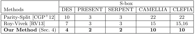
As a concrete application of our new method above, we show that for the generic higher-order masking of several well known S-boxes, e.g. DES, CLEFIA, PRESENT, etc., our method reduces the number of multiplications compared to the previously known methods [CGP+12,RV13]. In particular, using our method PRESENT can be masked with 2 multiplications (instead of 3), and DES with 4 multiplications (instead of 7), see Table 1. Our method achieves optimal com-plexity for the PRESENT S-box since it was proved in [RV13] that 2 non-linear multiplications are necessary to evaluate it. In Table 5, we report the timing results for DES masked using our technique.
S-box
Methods DES PRESENT SERPENT CAMELLIA CLEFIA
Parity-Split [CGP+12] 10 3 3 22 22
Roy-Vivek [RV13] 7 3 3 15 15,16
Our Method(Sec. 4) 4 2 2 10 10
Table 1.Number of non-linear multiplications required for the CGPQR generic higher-order masking scheme.
We also prove a lower bound ofΩ(2n/2/√n) for the complexity of any method to evaluaten-bit S-boxes, a.k.a.masking complexity; this shows that our method is asymptotically optimal. Our new lower bound significantly improves upon the previously known bound ofΩ(log2n) from [RV13].
2
Generic Polynomial Evaluation Technique
Before we describe our improved method to evaluate polynomials over F2n, let
us first recollect in Section 2.1 the method proposed by Roy and Vivek [RV13, Section 4] to evaluate the polynomials (over F26) corresponding to the DES
S-boxes. Their method requires 7 non-linear multiplications. The method in [RV13] is based on the Divide-and-Conquer strategy, which is an adaptation of a polynomial evaluation technique by Paterson and Stockmeyer [PS73]. The technique consists in decomposing the polynomial to be evaluated in terms of polynomials having their monomials from a precomputed set. Our method is partly based on this idea.
2.1 The Roy-Vivek Method for DES S-boxes
LetPDES(x)∈F26[x] be the Lagrange interpolation polynomial corresponding
with the elements ofF26. Note that for all the DES S-boxes, deg (PDES(x)) = 62.
Write
PDES(x) =q(x)·x36+R(x),
where deg(R)≤35 and deg(q) = 26. Then divide the polynomialR(x)−x27by
q(x):
R(x)−x27=c(x)·q(x) +s(x),
where deg(c)≤9 and deg(s)≤25, which gives
PDES(x) = x36+c(x)
·q(x) +x27+s(x).
Next decompose the polynomials q(x) and x27+s(x) in a similar way but, instead, dividing first by x18, and then usingx9 as the “correction term”. One gets
q(x) = (x18+c1(x))·q1(x) +x9+s1(x),
x27+s(x) = (x18+c2(x))·q2(x) +x9+s2(x)
where deg(q1) = 8, deg(c1) ≤ 9, deg(s1) ≤ 7, deg(q2) = 9, deg(c2) ≤ 8, and deg(s2)≤8. Finally,
PDES(x) =(x36+c(x))·
((x18+c1(x))·q1(x)) + (x9+s1(x))
+(x18+c2(x))·q2(x) + (x9+s2(x))
.
(2)
In [RV13], the monomials x, x2, x3, x4, x5, x6, x7, x8, x9, x18, x36 are first evaluated using 4 non-linear multiplications. Namely a non-linear multiplication is required for each of the monomialsx3,x5,x7andx9; the rest of the monomials can be evaluated using linear squarings only. Each of the individual polynomials in the above expression such as x36+c(x), x18+c
1(x), q1(x), and so on, can then be evaluated for free, that is without further non-linear multiplications. To evaluate PDES(x) from (2), 3 more non-linear multiplications are needed, and hence totally 7 non-linear multiplications are sufficient to evaluate a DES S-box. To sum up, the basic idea behind the above technique is to precompute a set of monomials, and then obtain a decomposition of the required polynomial in terms of polynomials having their monomials only from the precomputed set. Note that the said decomposition is obtained in a “fixed” way that depends only on the degree of the polynomial, which is required to be of the formk(2p−1)±c, for some parametersk,pandc; we refer to [RV13] for more details.
In the new method we propose next, we also precompute a set of monomials as above, but we also include every other monomial that can be computed for free by the squaring operation; that is we always generate the full cyclotomic class for any computed monomial. Then we try to decompose the polynomial as a sum of product of two polynomials having their monomials from the precomputed set. One of the two polynomials in every summand is randomly chosen, and we try to determine the other polynomial by solving (for unknown coefficients) the system of linear equations obtained by evaluating the polynomial at every point of the domain F2n. This approach of determining the unknown coefficients of
2.2 Our New Generic Method
Let us first recollect the notion of cyclotomic class overF2nand introduce some
notations. The cyclotomic class ofαw.r.t.n(n≥1 , 0≤α≤ 2n−2), denoted byCα, is defined as the set of integers
Cα=
α·2i (mod 2n−1) : i= 0,1, . . . , n−1 .
Intuitively,Cα corresponds to the exponents of all the monomials that can be computed fromxα∈F2n[x] using only the squaring operations (modulox2
n
+x). Since our goal is only to evaluate polynomials over F2n, we will be actually
working in the ring F2n[x]/(x2 n
+x), which is an abuse of the notationF2n[x].
In other words, we treat any polynomialP(x)∈F2n[x] to be the same asP(x)
modulox2n+x; henceP(x) has degree at most 2n−1.
By d ←$ D we denote an element d chosen uniformly at random from a set D. For any subset Λ⊆ {0,1, . . . ,2n−2}, xΛ denotes the set of monomials
xΛ =xi : i∈Λ ⊆F2n[x]. Finally we denote byP(xΛ) the set of all
polyno-mials inF2n[x] whose monomials are only from the setxΛ.
Description. Consider an n-bit to n-bit S-Box represented by a polynomial
P(x)∈F2n[x]. We consider a collectionS of` cyclotomic classes w.r.t.n:
S={Cα1=0, Cα2=1, Cα3, . . . , Cα`}. (3)
Also, defineLas the set of all integers in the cyclotomic classes ofS:
L= ∪ Ci∈S
Ci. (4)
We choose the setS of ` cyclotomic classes in (3) so that the set of corre-sponding monomials xL from S can be computed using only `−2 non-linear multiplications. We require that every monomialx0,x1,. . .,x2n−1
, can be writ-ten as product of some two monomials in P(xL). Moreover, we try to choose only those cyclotomic classes with the maximum number ofnelements (except
C0 which has only a single element). This gives
|L|= 1 +n·(`−1). (5) Next, we generatet−1 random polynomialsqi(x)
$
← P(xL) that have their monomials only in xL. Suitable values for the parameters t and |L| will be determined later. Then, we try to findt polynomialspi(x)∈ P(xL) such that
P(x) = t−1 X i=1
pi(x)·qi(x) + pt(x). (6)
theorem. More precisely, to find the polynomials pi(x), we solve the following system of linear equations overF2n:
A·c=b (7)
where the matrixAis obtained by evaluating the R.H.S. of (6) at every element ofF2n, and by treating the unknown coefficients ofpi(x) as variables. This matrix
has 2n rows andt· |L| columns, since each of thet polynomials p
i(x) has|L| unknown coefficients. The matrixAcan also be written as a block concatenation of smaller matrices:
A= (A1|A2|. . .|At), (8) where Ai is a 2n× |L| matrix corresponding to the product pi(x)·qi(x). Let
aj ∈ F2n (j = 0,1, . . . ,2n −1) be all the field elements and pi(x) consists of
the monomials xk1, xk2, . . . , xk|L| ∈ xL. Then, the matrix A
i has the following structure:
Ai =
ak1
0 ·qi(a0) a0k2·qi(a0) . . . a k|L|
0 ·qi(a0)
ak1
1 ·qi(a1) a1k2·qi(a1) . . . a k|L|
1 ·qi(a1)
ak1
2 ·qi(a2) a2k2·qi(a2) . . . a k|L|
2 ·qi(a2) ..
. ... . . . ...
ak1
2n−1·qi(a2n−1) ak2n2−1·qi(a2n−1) . . . a
k|L|
2n−1·qi(a2n−1)
(9)
The unknown vectorcin (7) corresponds to the unknown coefficients of the polynomialspi(x). The vectorbis formed by evaluatingP(x) at every element of
F2n. Note that sinceP(x) corresponds to an S-box, the vectorbcan be directly
obtained from the corresponding S-box lookup table.
If the matrixAhas rank 2n, then we are able to guarantee that the decom-position in (6) exists for every polynomialP(x). To be of full rank 2nthe matrix must have a number of columns≥2n. This gives us the necessary condition
t· |L| ≥2n. (10) We stress that (10) is only a necessary condition. Namely we don’t know how to prove that the matrixAwill be full rank when the previous condition is satisfied; this makes our algorithm heuristic. In practice for random polynomials
qi(x) we almost always obtain a full rank matrix under condition (10). From (5), we get the condition
t·(1 +n·(`−1))≥2n (11) where t is the number of polynomials pi(x) and ` the number of cyclotomic classes in the setS, to evaluate a polynomialP(x) overF2n.
earlier, we need`−2 non-linear multiplications to precompute the setxL. Hence the total number of non-linear multiplications required is then
Nmult=`−2 +t−1 =`+t−3. (12) where t is the number of polynomials pi(x) and ` the number of cyclotomic classes in the setS.
Algorithm 1New generic polynomial decomposition algorithm
Input: P(x)∈F2n[x].
Output: Polynomialspi(x), qi(x) such thatP(x) = t−1 P
i=1
pi(x)·qi(x) +pt(x).
1: Choose ` cyclotomic classes Cαi : L ←
l
S
i=1
Cαi, and the basis set x
L can be
computed using`−2 non-linear multiplications. 2: Choosetsuch thatt· |L| ≥2n.
3: For 1≤i≤t, chooseqi(x)
$
← P xL .
4: Construct the matrixA←(A1|A2|. . .|At), where eachAi is the 2n× |L|matrix
given by (9).
5: Solve the linear systemA·c=b, wherebis the evaluation ofP(x) at every element ofF2n.
6: Construct the polynomialspi(x) from the solution vectorc.
Remark 1. If A has rank 2n, then the same set of basis polynomials q
i(x) will yield a decomposition as in (6) foranypolynomial P(x). That is, the matrixA
is independent from the polynomialP(x) to be evaluated.
Remark 2. Our decomposition method is heuristic because for a givennin F2n
we do not know how to guarantee that the matrix Ahas full rank 2n. However for typical values of n, say n= 4,6,8, we can definitely check that the matrix
A has full rank, for a particular choice of random polynomialsqi(x). Then any polynomial P(x) can be decomposed using these polynomials qi(x). In other words for a given n we can once and for all generate the random polynomials
qi(x) and check that the matrix A has full rank 2n, which will prove that any polynomial P(x)∈ F2n[x] can then be decomposed as above. In summary our
method is heuristic for large values ofn, but can be proven for small values ofn. Such proof requires to compute the rank of a matrix with 2n rows and a slightly larger number of columns, which takesO(23n) time using Gaussian elimination. Asymptotic Analysis. Substituting (12) in (11) to eliminate the parameter`, we get
t·(1 +n·(Nmult−t+ 2))≥2n, =⇒ Nmult≥
2n
n·t +t−
2 + 1
n
The R.H.S. of the above expression is minimized whent≈q2n
n , and hence we obtain
Nmult≥2· r
2n
n −
2 + 1
n
. (14)
Hence, our heuristic method requiresO(p
2n/n) non-linear multiplications, whi-ch is asymptotically slightly better than the Parity-Split method [CGP+12], which has proven complexityO(√2n). If one has to rigorously establish the above bound for our method, then we may have to prove the following statements, which we leave as open problems:
• We can sample the collection S of cyclotomic classes in (3), each having maximal lengthn(other thanC0), using at most`−2 non-linear multipli-cations.
• The conditiont· |L| ≥2n suffices to ensure that the matrixAhas full rank 2n.
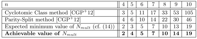
Table 2 lists the expected minimum number of non-linear multiplications, as determined by (14), for binary fields F2n of practical interest. It also lists
the actual number of non-linear multiplications that suffices to evaluate any polynomial, for which we have verified that the matrixAhas full rank 2n, for a particular random choice of theqi(x) polynomials. We also provide a performance comparison of our method with that of the Cyclotomic Class and the Parity-Split methods from [CGP+12]. Here we do not compare with the results from [RV13] since that work is mainly concerned with the optimization of specific S-boxes and polynomials of specific degrees; however such comparison will be made for specific S-boxes in Section 4. In Appendix B, we list the specific choice of parameters tandLthat we used in this experiment.
n 4 5 6 7 8 9 10
Cyclotomic Class method [CGP+12] 3 5 11 17 33 53 105 Parity-Split method [CGP+12] 4 6 10 14 22 30 46 Expected minimum value ofNmult (cf. (14)) 2 3 5 7 10 13 19
Achievable value of Nmult 2 4 5 7 10 14 19
Table 2.Minimum values ofNmult
Counting the Linear Operations. From (5) and (6), we get (2t−1)·(|L| − 1) + (t−1) as an upper-bound on the number of addition operations required to evaluateP(x). This is because each of the 2t−1 polynomialspi(x) andqi(x) in (6) have (at most)|L|terms, and there aretsummands in (6). From (10), we get:
Similarly, we get (2t−1)· |L| ≈2·2n as an estimate for the number of scalar multiplications. Since the squaring operations are used only to compute the list
L, we need|L| −`≤ |L| ≈√n·2n many of them (cf. (13)).
Remark 3. The above count of the linear operations can be significantly reduced if the linear operations are replaced by table lookups as much as possible. Such an approach is particularly well suited for application in the higher-order masking scheme of [CGP+12], where we need to evaluate a given polynomial with many shares and that the processing of linear polynomials with shares is particularly straightforward. More specifically, we can write eachpi(x) as a sum ofF2-linear
polynomials pi,j, one for each cyclotomic class in the pre-computed set S (cf. (3), (4)):
pi(x) = X Cαj∈S
pi,j(xαj).
The` polynomialspi,j are F2-linear and hence are of the form n−1
P k=0
γkx2
k
. Sim-ilarly, the polynomials qi(x) can also be expressed in the above form. If we tabulate the values of each of the linear polynomialspi,j andqi,j, then it suffices to evaluate xαj for each cyclotomic class C
αj ∈ S using only NLMs. Then the
polynomialspi,jandqi,jcan be evaluated by just table lookups, and then each of the 2t−1 polynomialspi andqican be eventually evaluated with`−1 additions each. Finally, we need t−1 more additions in the step (6). Hence, we need no scalar multiplications nor squarings using this table lookup technique. The total number of additions we need is
(2t−1)·(`−1) +t−1≈2·2 n
n .
Note that this technique is not very effective for the evaluation method of [RV13] since nearly every linear polynomial that appears has at most two non-zero terms.
3
New Lower Bound for Polynomial Evaluation
In this section, we show that our method from the previous section is asymp-totically optimal. More precisely, we show that to evaluate any polynomial over
F2n, any algorithm must use at leastO(p2n/n) non-linear multiplications. This
improves the previously known bound ofΩ(log2n) from [RV13].
To establish our lower bound we first need a formal model that describes polynomial evaluation over F2n. Such a model, the F2n-polynomial chain, has
been described in [RV13, Section 3]. For the sake of completeness, we briefly recollect the definition in Appendix A.
of non-linear multiplications necessary to evaluate a polynomial P(x), a.k.a.
non-linear complexity of P(x), as the maximum of the quantity necessary to evaluate its monomials. LetM(P(x)) denote the non-linear complexity ofP(x). IfP(x) corresponds to ann-bit S-boxS, thenM(P(x)) is also called themasking complexity of S.
Proposition 1. [[RV13], Proposition 3] Let P(x) :=P2i=0n−1aixi be a
polyno-mial inF2n[x]. Then
M(P(x))≥ max 0≤i<2n−1
ai6=0
mn(i),
where mn(i) is the length of the shortest cyclotomic-class (CC) addition chain
of iw.r.t.n.
The following result gives a lower bound on the value ofmn(i) in terms of the Hamming weight ofi.
Proposition 2. [[RV13], Proposition 1]mn(i)≥ dlog2(ν(i))e, whereν(i)is the
Hamming weight of the binary representation ofi (0≤i≤2n−2). Sinceν(2n−2) =n−1, hence polynomials having the monomialx2n−2
will have non-linear complexity at least log2(n−1). HenceΩ(log2n) is a lower bound on the number of necessary non-linear multiplications required to evaluate polyno-mials overF2n.
New Lower Bound. Our technique to prove the lower bound of Ω(p2n/n) on the non-linear complexity is similar to the one used in the proof of [PS73, Theorem 2]. But we would like to emphasize that their result is not applicable to our setting since they work over the integers and the cost model used there is different from the one used in our case.
Proposition 3. There exists a polynomialP(x)∈F2n[x]such thatM(P(x))≥
q 2n
n −2.
Proof. At a more abstract level, an F2n-polynomial chain evaluating P(x) ∈
F2n[x] that uses r non-linear multiplications (r≥0) can be equivalently
de-scribed as a sequenceZ of polynomialsz−1,z0,. . .,zr, where
z−1= 1,
z0=x,
zk = βk,−1+
k−1 X i=0 n−1 X j=0
βk,i,jz2
j
i ·
β0k,−1+
k−1 X i=0 n−1 X j=0
βk,i,j0 zi2j
(modx2n+x), (15) wherek= 1,2, . . . , r, βk,−1, βk,−0 1, βk,i,j, βk,i,j0 ∈F2n. Lastly,
P(x) =βr+1,−1+ r X i=0 n−1 X j=0
βr+1,i,jz2
j
i (modx 2n
where againβr+1,−1, βr+1,i,j ∈F2n. .
Since the squaring operation isF2-linear in F2n, and that x2 n
= x for all
x∈ F2n, it is easy to see that any polynomial that can be evaluated using at
mosttnon-linear multiplications will be of the form as given in (16).
The number of parametersβk,−1,βk,−0 1,βk,i,j,βk,i,j0 in (15) for a given value of k(k= 1, . . . , r) is 2·(k·n+ 1). In (16), the number of parameters βr+1,−1,
βr+1,i,j is (r+ 1)·n+ 1. Totally, the number of parameters are
(r+ 1)n+ 1 + r X k=1
2 (kn+ 1).
Since there are only|F2n|2 n
distinct polynomials inF2n[x] (i.e. up to evaluation),
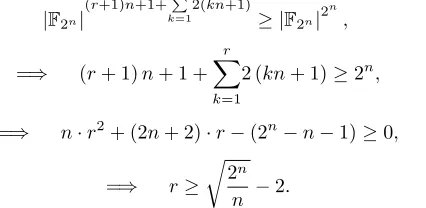
and a given set of values for the parameters enables to evaluate a single polyno-mial only, we get the following necessary condition to evaluate all polynopolyno-mials overF2n[x]
|F2n|
(r+1)n+1+Pr
k=1
2(kn+1)
≥ |F2n|2 n
,
=⇒ (r+ 1)n+ 1 + r X k=1
2 (kn+ 1)≥2n,
=⇒ n·r2+ (2n+ 2)·r−(2n−n−1)≥0,
=⇒ r≥ r
2n
n −2. (17)
Hence there exists polynomials overF2nthat requireΩ(p2n/n) non-linear
mul-tiplications to evaluate them. ut
The above proposition shows that our new method from Section 2.2 is asymp-totically optimal.
Concrete Lower Bound. In Table 3 we compare, for various values of n, the previously known lower bound for non-linear complexity with the new lower bound as determined by (17).
n 4 5 6 7 8 9 10 11 12
Previous lower bound [CGP+12,RV13] 2 2 3 3 4 4 4 4 4
Our lower bound(cf. (17)) 0 1 2 3 4 6 9 12 17
Table 3.Lower bound for non-linear complexity inF2n.
method the decomposition ofP(x) as
P(x) = t−1 X i=1
pi(x)·qi(x) +pt(x) (18)
is performed by first generating the polynomials qi(x) randomly and indepen-dently ofP(x), in order to have a linear system of equations over the coefficients of pi(x). Instead one could try to solve (18) for both the pi(x) and the qi(x) polynomials simultaneously; however this gives a quadratic system of equations, which is much harder to solve.
4
Application to various S-boxes
In this section, we apply the generic method described in Section 2, to several well known S-boxes. Using our new method, we reduce the number of non-linear multiplications required in each case, resulting in an improvement over the previously known techniques.
We stress that in our method for ann-bit S-box, the maximum number of non-linear multiplications required is invariant of the choice of the S-box when
nis fixed. Hence, the number of non-linear multiplications obtained for a fixed
n actually provides an upper bound on the masking complexity of an S-box of sizen.
4.1 CLEFIA and Other 8-bit S-boxes
The CLEFIA block cipher has two 8-bit S-boxes [SSA+07]. Let us denote the S-box lookup table for either of the S-boxes as Sclefia. We choose
L=C0∪C1∪C3∪C7∪C29∪C87∪C251. (19) This implies that after choosingt= 6, and then 5 basis polynomialsqi
$ ← P(xL) (1≤i≤5), the following system of equations is constructed inF28:
Sclefia[xj] = 5 X i=1
pi(xj)·qi(xj) | {z }
Q
+p6(xj) j = 0, . . . ,255. (20)
We have checked that for some random choice of the polynomialsqi(x) the corresponding matrix A has full rank 256, and therefore we can determine the polynomialspi(x). Given the solution to the above system, the S-box evaluation is then the same as evaluating the polynomial Q(x) +p6(x). To evaluate all the monomials in{x, x3, x7, x29, x87, x251}we need 5 non-linear multiplications, implying that any monomial in xL, any q
Therefore the total number of non-linear multiplications required for evaluating the S-box is 10.
Note that it requires at least 4 non-linear multiplications to evaluate the polynomials corresponding to the two S-boxes of CLEFIA by any method. This is because these two polynomials overF28 have degrees 252 (S-boxS0) and 254
(S-boxS1), and the result follows from Proposition 1.
Invariance. If we choose some other 8-bit S-box, then the matrix corresponding to the resulting system remains the same. Hence, we will still get a solution to the system for the same set of polynomialsqi(x). This implies that we can use the same set of basis polynomials to obtain polynomialspi(x) for any other 8-bit S-box. Hence, for any S-box of size 8, the number of non-linear multiplications is at most 10.
4.2 PRESENT and Other 4-bit S-boxes
For the 4-bit S-box of PRESENT [BKL+07], we choose t = 2 and L = C 0∪
C1∪C3. By selecting q1 $
← P(xL), we construct the following linear system of equations:
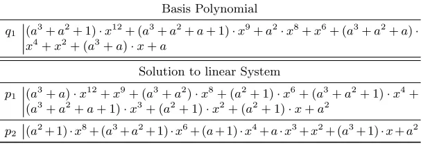
Spresent[xj] =p1(xj)·q1(xj) +p2(xj) (21) The monomials used to constructq1(x),q2(x) are{x, x2, x4, x8, x3, x6, x12, x9}. All of these monomials can be evaluated with a single non-linear multiplication and to evaluate p1(x)·q1(x) we need only one more non-linear multiplication. Hence, the PRESENT S-box evaluation requires 2 multiplications. As in the case of 8-bit S-boxes, this proves that with the same q1(x) any 4-bit S-box can be evaluated with 2 multiplications. Table 4 gives the corresponding polynomials for the PRESENT S-box.
The polynomial corresponding to the PRESENT S-box has degree 14 and hence, from Proposition 1, its masking complexity is at least 2 [RV13]. This im-plies that our evaluation method achieves optimal complexity for the PRESENT S-box.
4.3 (m, n)-bit S-box: Application to DES
We now consider S-boxes whose output size nis smaller than the input sizem, as for the DES S-boxes withm= 6 andn= 4. We can view an (m, n)-bit S-box (m > n) as a mapping fromF2m toF2n. Given any such S-box tableS, we want
to construct a system of linear equations
S[xj] = t−1 X i=1
pi(xj)·qi(xj) +pt(xj)
| {z }
G(x)
Basis Polynomial
q1 (a3+a2+ 1)·x12+ (a3+a2+a+ 1)·x9+a2·x8+x6+ (a3+a2+a)· x4+x2+ (a3+a)·x+a
Solution to linear System
p1 (a3+a)·x12+x9+ (a3+a2)·x8+ (a2+ 1)·x6+ (a3+a2+ 1)·x4+ (a3+a2+a+ 1)·x3+ (a2+ 1)·x2+ (a2+ 1)·x+a2
p2 (a2+ 1)·x8+ (a3+a2+ 1)·x6+ (a+ 1)·x4+a·x3+x2+ (a3+ 1)·x+a2
Table 4. Basis polynomial q1(x) for 4-bit S-boxes, and solutions p1(x), p2(x) to PRESENT S-box. The irreducible polynomial isa4+a+ 1 over
F2.
Note that each S[xj] is an element of the smaller field F2n, but each G(xj) is
an element in the larger fieldF2m. One trivial way to remove this inconsistency
is to considerS[xj] as an element of the larger fieldF2m, by padding the most
significant bit of the S-box output with 0’s. Then, we determine the polynomials
pi(x) by solving the corresponding system A·c = S, as described in Section 2.2. However intuitively this is not optimal, since we are creating an artificial constraint to be satisfied by the coefficients of the polynomials pi(x), namely that them−n most significant bits ofG(x) must be 0, while eventually these most significant bits will simply be discarded after the evaluation ofG(x), since to getS(x) we only keep thenleast significant bits ofG(x).
Instead, we consider the representations of the unknown coefficients of the polynomials pi(x) inF2 instead ofF2m, and we transform the system of linear
equations (22) over F2m, into a system of linear equations over F2. By doing
this, from each constraint G(xj), we generate m equations overF2, instead of
one equation over F2m. Note that each of these m equations will be an affine
combination of the unknown bits of the coefficients of the polynomials pi(x). Onlynof these equations are actually necessary, since the output of the S-box is of size nbits. By equating each of these equations to the corresponding output bit of the S-box, we get a transformed system of linear equations B·c = S, whereB is an (n·2m)×(t· |L| ·m) matrix overF2andLis the set of elements from the chosen cyclotomic classes. By solving this transformed system overF2 we determine the polynomialspi(x).
Example of DES. The DES block cipher has 8 (6,4)-bit S-boxes [oST93]. A DES S-box is a mapping from F26 to F24. In [RV13], the authors consider the
S-boxes as a mapping from F26 to F26, where the two most significant bits of
the output of S-box are fixed to 0, and as recalled in Section 2.1 the evaluation can be done with 7 non-linear multiplications. Also, for the same representation, there is a lower bound of 3 non-linear multiplications necessary to evaluate each DES S-box [RV13]. From Table 2, using our generic method over F26 we can
by working over F2 as explained above, only 4 non-linear multiplications are required.
We chooseL=C0∪C1∪C3∪C7, t= 3, and q1(x), q2(x) $
← P(xL). Then using our method we transform the following linear system of equations
Sdes[xj] = 2 X i=1
pi(xj)·qi(xj) | {z }
Q(x)
+p3(xj) (23)
to a system over F2. That is, instead of embedding Sdes intoF26, we write the
system of equations overF2. This can be done by considering the binary
repre-sentation of xα evaluated at any given value in
F26. This will give 6 equations
overF2for each equationQ(xj) +p3(xj). Out of these 6 equations only 4 will be necessary since the output of DES S-box has 4-bit values. By solving this new system of linear equations overF2 we can determinepi(x) for eachi.
The number of multiplications required to evaluateq1(x), q2(x) is 2, andQ(x) can be evaluated with 2 additional multiplications. Hence, the total number of non-linear multiplications required is only 4. In Appendix C we give an example of basis polynomials q1(x), q2(x) for DES and the solution polynomials pi(x) corresponding to the system of linear equations for the first DES S-box S1.
As previously, once we obtain a full rank matrix for a set of randomly fixed
q1(x), q2(x), for any other (6,4)-bit S-box we can use this basis to find the corresponding polynomials pi(x), since the matrix A is independent from the S-box. Hence we can conclude that the masking complexity of any (6,4)-bit S-box is at most 4.
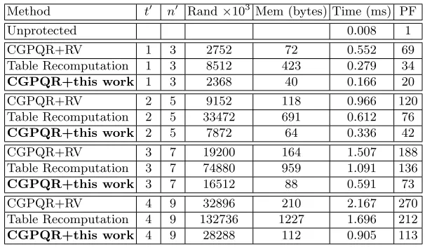
4.4 Implementation Results: DES
We have performed a software implementation of the CGPQR countermeasure [CGP+12] for DES that incorporates our new polynomial evaluation technique requiring only 4 NLMs. We have implemented this in C on a Dell Latitude 13 notebook running Ubuntu 12.04 Linux. The processor is Intel Core 2 Duo (32-bit architecture) running at 1.3 GHz. Our implementation is based on the source code available from [Cor13]. The present implementation is also publicly available at [Cor13]. We have used the technique of tabulating linear polynomials from Remark 3 in the implementation of our polynomial evaluation method. Note that these tables corresponding to the linear polynomials need to be stored only in the ROM.
time for a DES encryption is in milliseconds. The penalty factor (PF) gives the ratio of the execution time of a given method to that of an unprotected imple-mentation. The number of calls to the random number generator is 1000 times that of the reported quantity.
Table 5.Comparison of secure implementations of DES.
Method t0 n0 Rand×103 Mem (bytes) Time (ms) PF
Unprotected 0.008 1
CGPQR+RV 1 3 2752 72 0.552 69
Table Recomputation 1 3 8512 423 0.279 34
CGPQR+this work 1 3 2368 40 0.166 20
CGPQR+RV 2 5 9152 118 0.966 120
Table Recomputation 2 5 33472 691 0.612 76
CGPQR+this work 2 5 7872 64 0.336 42
CGPQR+RV 3 7 19200 164 1.507 188
Table Recomputation 3 7 74880 959 1.091 136
CGPQR+this work 3 7 16512 88 0.591 73
CGPQR+RV 4 9 32896 210 2.167 270
Table Recomputation 4 9 132736 1227 1.696 212
CGPQR+this work 4 9 28288 112 0.905 113
Acknowledgements
We would like to thank Matthieu Rivain for suggesting us the technique of tabulating linear polynomials described in Remark 3.
References
[BCO04] Eric Brier, Christophe Clavier, and Francis Olivier. Correlation power anal-ysis with a leakage model. In Marc Joye and Jean-Jacques Quisquater, editors,CHES, volume 3156 of Lecture Notes in Computer Science, pages 16–29. Springer, 2004.
[BKL+07] Andrey Bogdanov, Lars R. Knudsen, Gregor Leander, Christof Paar, Axel Poschmann, Matthew J. B. Robshaw, Yannick Seurin, and C. Vikkelsoe. Present: An ultra-lightweight block cipher. In Pascal Paillier and Ingrid Verbauwhede, editors,CHES, volume 4727 of Lecture Notes in Computer Science, pages 450–466. Springer, 2007.
[CGP+12] Claude Carlet, Louis Goubin, Emmanuel Prouff, Micha¨el Quisquater, and Matthieu Rivain. Higher-order masking schemes for S-Boxes. In Anne Can-teaut, editor,FSE, volume 7549 ofLecture Notes in Computer Science, pages 366–384. Springer, 2012.
[Cor14] Jean-S´ebastien Coron. Higher order masking of look-up tables. In Phong Q. Nguyen and Elisabeth Oswald, editors,Advances in Cryptology - EURO-CRYPT 2014 - 33rd Annual International Conference on the Theory and Applications of Cryptographic Techniques, Copenhagen, Denmark, May 11-15, 2014. Proceedings, volume 8441 ofLecture Notes in Computer Science, pages 441–458. Springer, 2014.
[CPRR13] Jean-Sebastien Coron, Emmanuel Prouff, Matthieu Rivain, and Thomas Roche. Higher-order side channel security and mask refreshing. In FSE, 2013. To appear.
[CRR02] Suresh Chari, Josyula R. Rao, and Pankaj Rohatgi. Template attacks. In Burton S. Kaliski Jr., C¸ etin Kaya Ko¸c, and Christof Paar, editors,CHES, volume 2523 ofLecture Notes in Computer Science, pages 13–28. Springer, 2002.
[GST13] Daniel Genkin, Adi Shamir, and Eran Tromer. RSA key extraction via low-bandwidth acoustic cryptanalysis. IACR Cryptology ePrint Archive, 2013:857, 2013.
[ISW03] Yuval Ishai, Amit Sahai, and David Wagner. Private circuits: Securing hard-ware against probing attacks. In Dan Boneh, editor,CRYPTO, volume 2729 ofLecture Notes in Computer Science, pages 463–481. Springer, 2003. [KJJ99] Paul C. Kocher, Joshua Jaffe, and Benjamin Jun. Differential power analysis.
In Michael J. Wiener, editor,CRYPTO, volume 1666 of Lecture Notes in Computer Science, pages 388–397. Springer, 1999.
[Mes00] Thomas S. Messerges. Using second-order power analysis to attack DPA resistant software. In C¸ etin Kaya Ko¸c and Christof Paar, editors,CHES, volume 1965 ofLecture Notes in Computer Science, pages 238–251. Springer, 2000.
[oST93] National Institute of Standards and Technology. FIPS 46-3: Data Encryp-tion Standard, March 1993. Available via csrc.nist.gov.
[PS73] Mike Paterson and Larry J. Stockmeyer. On the number of nonscalar multi-plications necessary to evaluate polynomials.SIAM J. Comput., 2(1):60–66, 1973.
[RP10] Matthieu Rivain and Emmanuel Prouff. Provably secure higher-order mask-ing of AES. In Stefan Mangard and Fran¸cois-Xavier Standaert, editors,
CHES, volume 6225 ofLecture Notes in Computer Science, pages 413–427. Springer, 2010.
[RV13] Arnab Roy and Srinivas Vivek. Analysis and improvement of the generic higher-order masking scheme of FSE 2012. In Guido Bertoni and Jean-S´ebastien Coron, editors,CHES, volume 8086 ofLecture Notes in Computer Science, pages 417–434. Springer, 2013.
[SSA+07] Taizo Shirai, Kyoji Shibutani, Toru Akishita, Shiho Moriai, and Tetsu Iwata. The 128-bit blockcipher CLEFIA (extended abstract). In Alex Biryukov, editor,FSE, volume 4593 ofLecture Notes in Computer Science, pages 181– 195. Springer, 2007.
A
F
2n-Polynomial Chain
Definition 1. [[RV13], Definition 4] An F2n-polynomial chain S for a
polyno-mial P(x)∈F2n[x]is defined as
where
λi=
λj+λk −1≤j, k < i,
λj·λk −1≤j, k < i,
αiλj −1≤j < i, αi is a scalar,
λ2
j −1≤j < i.
Though·andboth perform multiplication inF2n, the operator “” is reserved for the multiplication by a scalar. A step such as λj ·λk denotes a non-linear
multiplication. Let the number of non-linear multiplications involved in a chain
S be denoted as N(S). Then the non-linear complexity of P(x), denoted by
M(P(x)), is defined asM(P(x)) =min
S N(S).
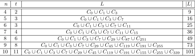
B
Heuristics for choosing parameters
t
and
L
n t L |L|
4 2 C0∪C1∪C3 9
5 3 C0∪C1∪C3∪C7 16
6 3 C0∪C1∪C3∪C7∪C11 25
7 4 C0∪C1∪C3∪C7∪C11∪C15 36
8 6 C0∪C1∪C3∪C7∪C29∪C87∪C251 49 9 8 C0∪C1∪C3∪C7∪C29∪C45∪C119∪C191∪C255 73 10 11 C0∪C1∪C3∪C7∪C29∪C45∪C119∪C191∪C155∪C255∪C339 101
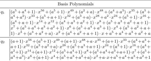
C
Evaluation Polynomials for DES S-boxes
Basis Polynomials
q1 (a5+a4+ 1)·x56+ (a5+ 1)·x49+ (a2+a)·x48+ (a4+a3)·x35+ (a5+ a4+a2)·x33+ (a5+a+ 1)·x32+ (a3+a)·x28+a2·x24+ (a5+ 1)·x16+ (a4+a+ 1)·x14+x12+ (a4+a3+a2+ 1)·x8+ (a5+a3+a2+a+ 1)· x7+ (a5+a4+a3+a2+ 1)·x6+ (a5+a4+a3+ 1)·x4+ (a5+a2+a+ 1)·x3+ (a3+a2+a)·x2+ (a4+a2+a+ 1)·x+a5+a4+a3+a2+a q2 (a+ 1)·x56+ (a5+ 1)·x49+ (a+ 1)·x48+a·x35+ (a+ 1)·x33+ (a4+a3+ a+1)·x32+(a3+a2+a)·x28+(a5+a3+a+1)·x24+(a3+1)·x16+(a4+ a2+1)·x14+(a+1)·x12+(a5+a4+1)·x8+(a5+a4+a3+a+1)·x7+(a5+ a4+a3)·x6+(a+1)·x4+(a5+a3+a2+a)·x2+a·x+a5+a4+a3+a2+1
Table 6.Basis polynomialsq1, q2 obtained fromP(xL), for DES.
Solution to linear system
p1 (a5+a4+a3+a2+1)·x56+(a5+a2+1)·x49+a4·x48+(a4+a3+a)·x35+ (a5+a4+a2)·x33+(a5+1)·x32+a·x28+(a4+a2)·x24+(a5+a)·x16+(a5+ a2)·x14+(a5+a+1)·x12+(a5+a4+a3+a)·x8+(a5+a4+a3+a)·x7+(a5+ a4+a3)·x6+(a2+a+1)·x4+(a5+a4+a)·x2+(a5+a4+1)·x+a4+a3+a2 p2 (a5+a2)·x49+ (a3+ 1)·x48+ (a5+a3+a+ 1)·x35+ (a4+a2+ 1)·
x33+ (a5+a4+ 1)·x32+ (a5+a4+a3+a+ 1)·x28+ (a3+a2)·x24+ (a2+a+ 1)·x16+ (a5+a4+a3)·x14+ (a4+a3+a+ 1)·x12+ (a4+ a3)·x8+ (a5+a)·x7+ (a5+a4)·x6+ (a5+a4+a3+a2+a+ 1)·x4+ (a5+a4+a)·x3+ (a5+a3+a+ 1)·x2+ (a5+a)·x+a5+a4+a2+a p3 a·x7+a·x6+ (a4+a+ 1)·x4+ (a5+a2+a)·x3+ (a5+a4+a+ 1)·
x2+ (a4+a2)·x
Table 7.Solution to the system of linear equations for DES S-box (S1). The irreducible polynomial isa6+a+ 1 over