A A Non-Parametric Algorithm for Discovering Triggering Patterns of Spatio-Temporal Event Types

A Non-Parametric Algorithm for Discovering

Triggering Patterns of Spatio-Temporal Event

Types

Berna Bakır Batu, Tuğba Taşkaya Temizel, and H. Şebnem Düzgün

Abstract—Temporal or spatio-temporal sequential pattern discovery is a well-recognized important problem in many domains like seismology, criminology and finance. The majority of the current approaches are based on candidate generation which necessitates parameter tuning namely, definition of a neighborhood, an interest measure and a threshold value to evaluate candidates. However, their performance is limited as the success of these methods relies heavily on parameter settings. In this paper, we propose an algorithm which uses a nonparametric stochastic de-clustering procedure and a multivariate Hawkes model to define triggering relations within and among the event types and employs the estimated model to extract significant triggering patterns of event types. We tested the proposed method with real and synthetic data sets exhibiting different characteristics. The method gives good results that are comparable with the methods based on candidate generation in the literature.

Index Terms—Diggle D, Hawkes self-exciting process, multivariate Hawkes model, space-time clustering, spatio-temporal sequences, stochastic declustering.

——————————  ——————————

1 I

spatio-temporal triggering pattern of event types is a sequence of spatio-temporal events where a former event generates the one that is following it. A spatio-temporal event is defined by the time and location at which the event took place with its type. An extracted spatio-temporal triggering pattern may reveal interesting relationships among the event types. An example scenar-io of a triggering pattern including six event types is rep-resented in Fig. 1. In the figure, discount day (DD) and concert (C) events at a shopping mall are the triggering (random) events, which trigger violating parking rules (VPR), pickpocketing (P) and clogging (CL) events. CL events further trigger fainting (F) events. Here, VPR is the common consequence of DD and C events; however, both ancestors can trigger the consequence individually. An event of the type triggered may be a casual event. A trig-gering event increases the likelihood of the triggered one. In other words, a triggered event type arises with a higher rate than usual after its triggering event type was ob-served. Lets assume that a VPR event occurs randomly with a specific mean rate. When a C event takes place at a specific time and location, we may observe more VPR events than usual within the neighborhood of the C event. In the literature, little attention has been paid to

discovery of the spatio-temporal sequential pattern of event types although temporal sequential patterns and spatial patterns have been extensively studied for decades (See, for example, [1], [2], [3]).

In this study, we propose an algorithm where we model relationship between events by using multivariate Hawkes model, which is a class of mutually exciting point process, in order to discover triggering patterns of spatio-temporal event types. We adapted stochastic de-clustering methodology with multivariate Hawkes model to estimate the mean rate of a cluster process by using the conditional intensity model. The model assumes that the process consists of events that occur randomly with a mean rate and events triggered by these random events. The conditional intensity of the process is the intensity at a particular time and location including both random and triggered events. Specifically, the conditional intensity model is known as self-exciting or Hawkes model which has a branching structure [4]. A typical application of the stochastic declustering methodology is to form earth-quake catalogue by discriminating mainshocks and after-shocks probabilistically [5], which utilizes parametric and nonparametric approaches based on the space-time branching models. The proposed methodology is based on the model independent stochastic declustering algo-rithm (MISD) [6]. Unlike the earthquake studies, in many domains, a parametric model defining the process’ branching structure is unknown. A non-parametric ap-proach may aid to give insight about the overall process. Based on several experiments on the earthquake data, Marsan and Lengline [6] demonstrated that MISD algo-rithm is able to find the causal structure of the process without any prior model. In this study, our main focus is xxxx-xxxx/0x/$xx.00 © 200x IEEE Published by the IEEE Computer Society

A

————————————————

 B. Bakır Batu is with the Department of Computer and Instructional Sciences Technology, Atatürk University, 25030, Erzurum, Turkey. E-mail: [email protected]

 T. Taşkaya Temizel is with the Department of Information Systems, Informatics Institute, Middle East Technical University, 06530, Ankara, Turkey.

E-mail: [email protected]

 H. Ş. Düzgün is with the Department of Mining Engineering, Middle East Technical University, 06530, Ankara, Turkey.

stationary cluster processes. The main contributions of this paper are as follows:

1. Our proposed approach does not require candi-date generation; instead it calculates triggering probabilities between the pairs of event instances and the probabilities for being a random or trig-gered event. Based on these values, it extracts in-teresting sequential patterns from data. We per-form rank selection to identify significant pairs within the extracted patterns and use pairwise triggering probabilities to calculate interest meas-ure.

2. Unlike existing algorithms, it does not require a neighbourhood definition since the interaction is explained by the spatio-temporal density function of distances. It is non-parametric since the pro-posed algorithm does not require a parametric density function such as Gaussian. The level of discretization used to estimate the density func-tion has an effect on the pairwise triggering prob-abilities, thus, interestingness (hereafter called sig-nificance in this text) of patterns may differ based on the discretization level chosen. We empirically handle this influence with Diggle D-function [7] which explores possible space time clustering or interaction with respect to separation distances. If the discretization level corresponds to spatio-temporal interaction range suggested by D-function for a given pairwise pattern, the pro-posed algorithm produces the highest probability for the pattern. As the smaller or larger ranges are used, the pattern probabilities decrease. On the contrary, one can use the algorithm for different discretization levels and find the interaction scale of the extracted patterns as the discretization val-ues that maximizes the pattern probability. 3. We adapted stochastic declustering methodology

in sequential pattern mining problem which is a new approach in this domain. In addition, we em-ploy multivariate spatio-temporal Hawkes model in the algorithm while previous studies have used univariate models which are limited to model only single type events.

2 R

W

Sequential pattern mining studies can be found in both temporal and spatio-temporal domains. In temporal do-main, pattern matching problem has been extensively studied after it was first introduced in [1] to extract se-quential patterns in customer transaction databases. Spa-tio-temporal analysis of point pattern is a more recent topic compared to the extensive studies on spatial point patterns analysis. In these studies, taking snapshots of time is a popular approach however it has some draw-backs [3], [8], [9]. The main drawback is the possibility to miss patterns at different time granularities; therefore, domain knowledge is essential in order to choose an ap-propriate discretization. In the context of spatio-temporal sequential pattern mining, most of the studies focus on object trajectory problem, which deals with the move-ment of the same object to find frequent routes followed by an object [10] or to detect motion flow in video streams [11]. These studies are relevant but different from our problem in a variety of aspects. The main difference is that moving object studies deal with how the location of the same object changes over time assuming that se-quences are the consecutive locations of the same object whereas, in this study, sequences consist of different ob-jects or event types which are realized in one location and do not move such as traffic accident at a particular loca-tion and time. In some papers, moving object problem is handled by event-based approaches. For example, Hornsby and Cole [12] model the dynamic objects such as automobiles, planes, boats, etc. in geospatial domain to track the movement of the objects by using an event-based approach. Colocation studies usually operate on spatial domain and aim to identify different spatial fea-tures frequently located together. This relationship can be measured by cross-K function or mean nearest neighbour distance [13]. An extension of colocation patterns in spa-tio-temporal domain is conducted by Çelik et al. [9], which investigates patterns at different time slots. Their study deals with the co-located objects which are moving in space together such as kicker or holder in a football match. Time is involved as snapshots and their method employs candidate generation approach with a proposed interest measure.

Studies similar to or directly related to the focus of our problem are very limited. An analysis of spatio-temporal sequence of different event types can be found in two studies [14], [15]. The main contributions of these studies are the proposed interestingness measures and mining algorithms which are suitable for spatio-temporal event data. Both studies use candidate generation approach. In [14], a framework is proposed for mining event-based spatio-temporal sequences. They define a follow predi-cate to identify sequences based on a spatio-temporal neighbourhood which is bounded by user specified thresholds and a significance measure called sequence index to determine significant sequences. The sequence index can be interpreted as cross-K function; however, it is a more generic measure since it allows incorporation of a temporal predicate and inclusion of more than two types. It is calculated based on the average density ratio Fig. 1. An example scenario for the triggering pattern of event types.

of subsequent events in the given neighbourhood relative to its overall density within the whole space. This pre-vents a sequence to be significant just because of the high density of an individual event. They also give the dynam-ic neighbourhood definitions such as a spatial neighbour-hood which is a function of time as well as different neighbourhood definitions for different event types. Mo-han et al. [15] aim to identify cascading events in an event dataset over a common spatio-temporal framework and extend the sequence discovery problem for partially or-dered patterns. They propose an algorithm for mining cascading spatio-temporal patterns (CSTP) and filtering strategies to prevent generating uninteresting candidates. They define a new significance measure called cascade participation index (CPI) which is the minimum of partic-ipation ratios of each event type in the sequence. They define participation ratio of an event type in a sequence as conditional probability of the sequence given a partici-pating event type. It is estimated as the number of in-stances of the event type participating in the sequence over the number of instances of the event type in the da-tabase. It is shown that CPI is an upper bound for the space-time K-function. The authors state that their focus is to improve computational performance of the CSTP algorithm, hence they do not address the effect of the pa-rameter choice such as neighborhood and significance measure thresholds and grid cell size defined for filtering. As a summary, a great majority of temporal and spa-tio-temporal sequence studies use a window-based ap-proach to define closeness of events or objects in time and space. The window is constant and bounded by a user specified threshold. All the events falling in the same window are considered as neighbours. Small threshold values may result in missing the true patterns at larger scales whereas higher values may produce irrelevant pat-terns. In addition, the time distances between events in a window are treated as the same and contribute to the sig-nificance measures such as support count equally while the ones larger than the threshold have no contribution. The window based neighbourhood definition may be suitable for some domains, such as DNA or character se-quences; however, it is not a realistic assumption in some other domains where the events of a sequence interact with each other according to a decay law. For instance, a main shock earthquake produces its aftershocks with a decreasing influence as time passes. A time window can-not capture the true relations in such sequences. Candi-date generation is a common approach in sequential pat-tern mining, yet it poses a challenge of exponential in-crease in the number of candidate patterns with respect to the number of types. In some studies such as [15], a num-ber of filtering strategies are used to tackle this challenge. Generally the number of windows in which a specific pattern is observed gives the support value for that pat-tern. The minimum support value is also required to be specified and should be provided by domain experts. Another limitation is the necessity of examining individ-ual distribution of event types or elements in a sequence before performing a mining task. A frequent sequence is not necessarily a meaningful pattern. For example, two

regular events may be observed in a time window long enough to include both with a specific order although their occurrences are independent. Furthermore, a fre-quent event sequence extracted by measures such as sup-port does not necessarily imply a triggering or causal re-lationship between event types although time order is a clue about causal relationship. We may not know if the preceding event triggers the next one in the sequence, rather we know how likely this sequence is observed. In fact, these shortcomings have significant importance if the sequential pattern mining problem aims to discover se-quential triggering relationship.

3 T

P

M

:

T

P

E

M

-T

S

-T

E

(TPEX)

In this section, we give relevant background information about the Hawkes model and MISD algorithm which we use as a base in TPEX algorithm. Then we present TPEX algorithm in detail.

3.1 Background: Hawkes Model and MISD Algorithm

A Hawkes point process defines the random events which are either an immigrant or a descendant. It was first introduced in [4] for temporal domain with possible application areas such as epidemiology and modelling neuron firing. The process has an underlying branching structure if the event locations are discarded; it is reduced to a simple branching process consisting of immigrants and descendants.

Univariate Hawkes model can be defined by the inten-sity function conditioned on the history Ht of the process at time t. It is assumed that some events in the process occur independently or as a result of an outside system with a mean rate 𝜇 and the value of 𝜇 can be considered as a constant or depends only on the location. Intensity at a particular location and time, (s, t), depends on both the mean rate and the previously occurred events with some degree based on the spatio-temporal distance of point (s,

t) to these historical events. The definition of the intensity

for an unmarked point process is given as; 𝜆(𝑠, 𝑡|𝐻_𝑡) = 𝜇 + ∑ 𝑔(𝑠 − 𝑠𝑗, 𝑡 − 𝑡𝑗; Θ)

𝑗:𝑡𝑗<𝑡

(1) In the equation (1), 𝑔(𝑠, 𝑡; 𝛩) is the triggering function of the process where  represents the distribution parame-ters. Besides the univariate case, Hawkes also proposes models for mutually-exciting point processes and exam-ines a special case where the decay is exponential. Multi-variate model generalizes the uniMulti-variate case by defining a conditional intensity for each component or event type k as follows:

𝜆_𝑘(𝑠, 𝑡|𝐻𝑡) = 𝜇𝑘+ ∑ ∑ 𝜂𝑟𝑘𝑔𝑟𝑘(𝑠 − 𝑠𝑗, 𝑡 − 𝑡𝑗; Θ) 𝑗:𝑡𝑗<𝑡

𝑟 (2)

where rk is the average number of event type k triggered by event type r, grk is the triggering function for the pairs of event types r and k which defines the probability of an

event type of r at (sj, tj) triggering an event type k at (s, t). The univariate Hawkes model with or without marks is employed in many studies, for example, to analyze earthquakes and crime events [5], [16], and to model tem-poral triggering behaviour of activities in social media such as Twitter and Wikipedia [17]. It becomes popular in seismological studies after Ogata [18] introduces Epidem-ic Type Aftershock Sequences (ETAS) model to predEpidem-ict earthquakes with marked Hawkes point process (See for example, [5], [19], [20]). ETAS model has also been ex-tended in both temporal and spatio-temporal domain where the earthquake occurences are described by a marked self-exciting (or branching) point process which is defined in space, time and magnitude. Each process con-sists of mainshock (background) and aftershock events where background events occur independently according to a mean rate µ(𝑥, 𝑦) with magnitudes M distributed in-dependently of µ. Based on the branching structure, each event increases the risk of aftershocks. The probability of the risk is defined by a kernel 𝑔(𝑠, 𝑡, 𝑀). Zhuang et.al [5] introduced stochastic declustering algorithm to discrimi-nate main shock earthquakes from their aftershocks by utilizing univariate Hawkes model with parametric trig-gering function which is estimated by maximum likeli-hood estimation (MLE) method through an iterative pro-cedure. In seismological science, there are well-developed parametric aftershock models for triggering function 𝑔 which can be used in conditional intensity model. In many other application domains, however, there is no prior information about the form of decay function which describes the triggering behavior. Even in seismology, aftershock effect can be more complicated due to second generation aftershocks produced by the previous after-shocks. As a remedy, Marsan and Lengline [6] propose a nonparametric approach called model independent sto-chastic declustering algorithm (MISD). This model is later used in crime analysis to estimate the mean rate of crime events and to identify dense areas as an alternative to the hot spot analysis which is the most common approach in this domain [21].

The MISD algorithm use univariate Hawkes model and estimate the conditional intensity and the mean rate with a nonparametric kernel estimation procedure. It as-sumes linearity of the triggering process. Since the branching structure is unobservable, in other words, we do not know which event actually triggers the others, the algorithm utilizes Expectation-Maximization method. The random variable Xij is defined for the branching structure and it takes value of 1 if ith _{event is caused by j}th _event, otherwise it takes the value of 0. Similarly, the random variable Xii takes the value of 1 if it is a triggering casual event; otherwise it takes the value of 0. Since these varia-bles cannot be observed, their expected values are esti-mated. The triggering function 𝑔 in (1) is replaced with nonparametric kernel estimate. Given nonparametric in-tensity model, the MISD algorithm works as follows:

Step 1: Start with the initial values for the intensity and

the mean rate.

Step 2: Calculate the expected values for the triggering

and the background probabilities as follows:

𝑝𝑖𝑗= { 𝑔(𝑠𝑖− 𝑠𝑗, 𝑡𝑖− 𝑡𝑗) 𝜆(𝑠, 𝑡\𝐻_𝑡) , 𝑡𝑖> 𝑡𝑗 0, 𝑜𝑡ℎ𝑒𝑟𝑤𝑖𝑠𝑒 (3) 𝑝𝑖𝑖= 𝜇 𝜆(𝑠, 𝑡\𝐻𝑡) (4) where, 𝜆 is intensity defined in (1), pij is the probability of the ith _{event being triggered by the j}th _{event and pii is the} probability of ith _{event being a background event.}

Step 3: Update the intensity and the mean rate based

on the probabilities calculated in the expectation step as follows: 𝑔(∆𝑠, ∆𝑡) = 1 𝛿𝑠 × 𝛿𝑡 ∑ 𝑝𝑖𝑗 𝑖,𝑗∈Λ (5) 𝜇 = 1 𝑇 × 𝑅∑ 𝑝𝑖𝑖 𝑛 𝑖=1 (6)

where s,t are the discretization parameters,  is the set of pairs such that 𝑡𝑖− 𝑡𝑗 𝜖 [𝑡 − 𝛿𝑡, 𝑡 + 𝛿𝑡) and 𝑠𝑖− 𝑠𝑗 𝜖 [𝑠 −

𝛿𝑠, 𝑠 + 𝛿𝑠), T is the duration of time, R is the area of the studied region and n is the number of events. Step 2 and Step 3 are repeated until g and μ converge.

3.2 TPEX Algorithm

We propose that self-exciting Hawkes models can be used for sequential pattern mining where the elements of the

patterns are related based on a

caus-al/branching/triggering structure. A cause/triggering event can be considered as a mainshock earthquake whereas an effect/a triggered event can be assumed as an aftershock. Triggered events form a cluster around its triggering event(s). Therefore, self exciting models can be used to define events in any domains if the events are generated based on a branching structure and the entire process consists of clustered process and independent cause events. Moreover, if the process consists of different event types, a multivariate model explains branching structure better. Multivariate temporal models have re-ceived significant attention in the recent years. Embrechts, et.al. [22] conduct a study on financial data to investigate triggering effect on extremes. Zhou and Zha [23] propose an algorithm for learning kernel functions of multivariate Hawkes processes. Some recent studies are carried out by using multivariate Hawkes models to learn temporal triggering behavior of users in social networks [24], [25]. To the best of our knowledge, there is no study yet deal-ing with spatio-temporal multivariate Hawkes model.

TPEX algorithm finds pairwise triggering patterns of spatio-temporal event types. The pseudocode of the algo-rithm is given in Algoalgo-rithm 1. It first fits conditional in-tensity model by using non-parametric multivariate Hawkes process and calculates pairwise probabilities for all pair of instances (Line 1-4). It then selects significant probabilities with rank selection method and generate distinct pairwise patterns from this reduced set. 𝜀 is a threshold value which is used to ensure selection of prob-abilities which are very close to the maximum pairwise probability value in a row (Line 5-8). It returns each sig-nificant pattern with its interest measure (Line 9-10). A spatio-temporal dataset consisting of locations and the

types of the events and the discretization values for the density functions are the inputs of the algorithm. Stop-ping criterion is satisfied by the convergence of the mean rate and density functions which also ensures conver-gence of probabilities.

We define conditional expectations for the random var-iables 𝑋𝑖𝑗 and 𝑋𝑖𝑖 with respect to the type of the events

and adapt the MISD algorithm for the multivariate mod-el. Let Y be a discrete random variable representing the type of a spatio-temporal event occurred at a particular time t and location s. Assume that the sample space of Y consists of K number of event types and there are n number of observa-tions, 𝑦1, 𝑦2, … , 𝑦𝑛 of Y. We define the following random

variables conditioned on the value of Y. 𝑋𝑖𝑗|𝑌𝑖, 𝑌𝑗= { 1, 𝑖𝑓 𝑖𝑡ℎ _{𝑒𝑣𝑒𝑛𝑡 𝑖𝑠 𝑐𝑎𝑢𝑠𝑒𝑑 𝑏𝑦} 𝑗𝑡ℎ _{𝑒𝑣𝑒𝑛𝑡 𝑔𝑖𝑣𝑒𝑛 𝑌} 𝑖, 𝑌𝑗 0, 𝑜𝑡ℎ𝑒𝑟𝑤𝑖𝑠𝑒 (7) 𝑋_𝑖𝑖|𝑌_𝑖= { 1, 𝑖𝑓 𝑖𝑡ℎ _{𝑒𝑣𝑒𝑛𝑡 𝑜𝑐𝑐𝑢𝑟𝑠} 𝑟𝑎𝑛𝑑𝑜𝑚𝑙𝑦 𝑔𝑖𝑣𝑒𝑛 𝑌𝑖 0, 𝑜𝑡ℎ𝑒𝑟𝑤𝑖𝑠𝑒 (8) Then, the conditional expectations are calculated using conditional densities, 𝐸(𝑋𝑖𝑗|𝑌𝑖, 𝑌𝑗) = 𝑃(𝑋𝑖𝑗|𝑌𝑖, 𝑌𝑗)

and 𝐸(𝑋𝑖𝑖|𝑌𝑖) = 𝑃(𝑋𝑖𝑖|𝑌𝑖). The spatio-temporal conditional

intensity functions for each event type 𝑘 where 𝑘 = 1, 2, … , 𝐾 can be defined by multivariate Hawkes model as follows: 𝜆𝑘(𝑠, 𝑡|𝐻𝑡) = 𝜇𝑘+ ∑ ∑ 𝑓𝑟𝑘(𝑠 − 𝑠𝑗, 𝑡 − 𝑡𝑗) 𝑗:𝑡𝑗<𝑡 𝑌𝑗=𝑟 𝐾 𝑟=1 (9)

where 𝑓𝑟𝑘(𝑠, 𝑡) = 𝜂𝑟𝑘𝑔𝑟𝑘(𝑠, 𝑡), and it is estimated by using

histogram estimator defined in (12). Note that MISD is analogous to histogram density estimation [26]. We as-sume constant mean rate for each event type. Given the nonparametric multivariate conditional intensity model in (9), we estimate conditional probability distribution of random variables 𝑋𝑖𝑗 and 𝑋𝑖𝑖 by modifying equations in Step 2 and Step 3 given in Section 3.1 as follows:

𝑝′ 𝑖𝑗= 𝑃(𝑋𝑖𝑗|𝑌𝑖, 𝑌𝑗) = 𝑓𝑌𝑗𝑌𝑖(𝑠𝑖− 𝑠𝑗, 𝑡𝑖− 𝑡𝑗) 𝜆𝑌𝑖(𝑠𝑖, 𝑡𝑖|𝐻𝑡𝑖) (10) 𝑝′ 𝑖𝑖= 𝑃(𝑋𝑖𝑖|𝑌𝑖) = 𝜇𝑌𝑖 𝜆_𝑌𝑖(𝑠_𝑖, 𝑡_𝑖|𝐻_𝑡𝑖) (11) 𝑓_𝑟𝑘(∆𝑠, ∆𝑡) = 1 𝑁𝑟𝑘× 𝛿𝑠 × 𝛿𝑡 ∑ 1_{𝑌𝑖=𝑘,𝑌𝑗=𝑟}× 𝑝_𝑖𝑗 𝑖,𝑗∈𝛬 (12) 𝜇𝑘= 1 𝑁_𝑘× 𝑇 × 𝑅∑ 1𝑌𝑖=𝑘× 𝑝𝑖𝑖 𝑛 𝑖=1 (13)

where T is the duration of time, R is the area of the study region, 1 is the indicator function, n is the number of ob-served events, Nrk is the number of pairs of type (𝑌𝑖=

𝑘, 𝑌𝑗= 𝑟) where 𝑡𝑖 > 𝑡𝑗, 𝑁𝑘 is the number of observed

events of type 𝑘, 𝑠 and 𝑡 are the discretization parame-ters and  is the set of pairs such that 𝑡𝑖− 𝑡𝑗 𝜖 [𝑡 − 𝛿𝑡, 𝑡 +

𝛿𝑡) and 𝑠𝑖− 𝑠𝑗 𝜖 [𝑠 − 𝛿𝑠, 𝑠 + 𝛿𝑠).

An event occurred at a particular time and location is either a random event or a triggered event by one or more former events. 𝑝′

𝑖𝑗 shows the proportion of the triggering

level between the two events whereas 𝑝′

𝑖𝑖 shows the

pro-portion of the mean rate in the intensity model. If jth _event triggers ith _{event, their triggering level defined by the 𝑓} function (12) produces a higher score consequently mak-ing 𝑝′

𝑖𝑗 (10) high. Similarly, if ith event occurs randomly,

the total triggering level between the ith _{event and each j}th event, where tj<ti and j=1, 2,…, i-1, will be low which ap-proximates the value of lambda to the mean rate and the value of 𝑝′

𝑖𝑖 (11) to 1. For a given ith event, the sum of the

𝑝′

𝑖𝑗 and 𝑝′𝑖𝑖 for all tj<ti is equal to 1.

Our primary assumption for the pairwise relationship is that if there is an interaction at a particular scale, there should be many pairwise space-time distances less than the maximum interaction range while other distance val-ues are evenly distributed. The estimated density function will reflect this relationship with peaks if appropriate discretization values are utilized. There may be different scales where space-time interaction exists. Large discreti-zation intervals may suppress the relation at smaller scales, therefore, performing multiple runs with different discretization values is worthy. We can also explore and test significant space-time clusters at different scales with

D-function and supervise the estimation with these

val-ues. In the analysis of spatio-temporal dependence Diggle et al. [7] use Ripley's K-function as a diagnostic tool and ex-plore significant space-time clusters with D-function:

𝐷(𝑠, 𝑡) = 𝐾(𝑠, 𝑡) − 𝐾(𝑠)𝐾(𝑡) (14)

where 𝐾(𝑠, 𝑡), 𝐾(𝑠) and 𝐾(𝑡) are Ripley's K-function [27] (or second order moment measure) in spatio-temporal, spatial and temporal domain, respectively. If there is no space-time interaction or clustering, the two terms in the right hand side of the Equation (14) is identical, and thus,

D-Algorithm 1 Triggering Pattern Extraction (TPEX) Algorithm Input: 1) 𝐷𝑎𝑡𝑎 = {(𝑠𝑖, 𝑡𝑖, 𝑦𝑖)| 𝑖 ∈ (1,2, … , 𝑛), 𝑠𝑖 ∈ 𝑅2, 𝑡𝑖 ∈ 𝑅, 𝑦_𝑖∈ (1,2, … , 𝐾)}. 2) Discretization values: δs, δt. Output:

Pairwise triggering patterns and their signifi-cance: 𝑇𝑃 = {(𝑟 → 𝑘, 𝑠𝑖𝑔𝑛𝑖𝑓𝑖𝑐𝑎𝑛𝑐𝑒𝑟→𝑘)}

Algorithm:

1: Initialize 𝜇𝑘 and 𝑓𝑟𝑘, 𝑟, 𝑘 ∈ (1,2, … , 𝐾)

2: while 𝜇 and 𝑓 not converged do

3: Calculate 𝑝′𝑖𝑗 and 𝑝′𝑖𝑖 from (10) and (11)

4: Update 𝜇𝑘 and 𝑓𝑟𝑘 from (12) and (13)

5: 𝑃𝑎𝑖𝑟 𝑃𝑟𝑜𝑏𝑎𝑏𝑖𝑙𝑖𝑡𝑖𝑒𝑠 = ∅ 6: for each 𝑖 ∈ (1,2, … , 𝑛) 7: 𝑃𝑎𝑖𝑟 𝑃𝑟𝑜𝑏𝑎𝑏𝑖𝑙𝑖𝑡𝑖𝑒𝑠 = 𝑃𝑎𝑖𝑟 𝑃𝑟𝑜𝑏𝑎𝑏𝑖𝑙𝑖𝑡𝑖𝑒𝑠 ∪ { (𝑖, 𝑗, 𝑝𝑖𝑗∗) | 𝑝𝑖𝑗∗= max(𝑝′_𝑖1, 𝑝′_𝑖2, … , 𝑝′_𝑖𝑖) ∨ max(𝑝′ 𝑖1, 𝑝 ′ 𝑖2, … , 𝑝 ′ 𝑖𝑖) − 𝑝𝑖𝑗 ∗_{< 𝜀}}

8: Determine set of distinct patterns 𝑟 → 𝑘 from 𝑃𝑎𝑖𝑟 𝑃𝑟𝑜𝑏𝑎𝑏𝑖𝑙𝑖𝑡𝑖𝑒𝑠

9: Calculate 𝑠𝑖𝑔𝑛𝑖𝑓𝑖𝑐𝑎𝑛𝑐𝑒𝑟→𝑘=

𝑚𝑖𝑑𝑚𝑒𝑎𝑛(𝑝𝑖𝑗∗ | 𝑦𝑗= 𝑟, 𝑦𝑖 = 𝑘) from (15)

function is equal to 0. If there is an interaction, the surface of 𝐷(𝑠, 𝑡) shows peaks at the corresponding ranges. If this in-formation supervised the algorithm as discretization val-ues, TPEX produces optimal results in terms of signifi-cance and rank values for a certain group of patterns in-teracting at similar scales. High discretization values may result in missing patterns at small scales; on the other hand, small discretization values may cause a decrease in significance values of patterns at larger scales.

We evaluate the significance of the resulting patterns by extracting patterns of event types from the pair of in-stances, which are obtained by performing rank selection. Each pair of instances contributes to a pattern with a probability value. In our experimental study, we realized that the distribution of the estimated probabilities for a particular pattern is not normal; instead it usually shows heavy-tailed and left-skewed distribution. Mosteller and Tukey [28] discuss the robustness of the location measures in terms of two concepts when the data is not normal. Robustness of validity ensures that regardless of the underlying distribution the confidence interval for the population location will cover the true value with a 95% of chance. Robustness of efficiency means that confidence interval for the population location is as narrow as the one we can have when the true shape of the distribution is known. The mean and the median are the best in terms of these two robustness measures when the data is nor-mal. However, in the case of non-normality, the robust-ness of validity does not hold for the mean whereas the median lacks robustness of efficiency. In order to mini-mize this trade off we use mid-mean as a location meas-ure for the pair probabilities. The probability of a trigger-ing pattern of two types is the mid-mean of the probabil-ity values of the pair of instances, which constitute the pattern. It can be written as:

𝑃(𝑟 → 𝑘) = 𝑚𝑖𝑑𝑚𝑒𝑎𝑛(𝑝∗

𝑖𝑗: 𝑌𝑗→ 𝑌𝑖 = 𝑟 → 𝑘) (15)

where 𝑝∗

𝑖𝑗 is the probability of the pair of instance which

contributes to the pattern.

To illustrate the algorithm lets consider a toy example with four data samples: {(x, y, t, type): (5, 7, 1, A), (3, 8, 2.1, B), (7, 4, 2.5, B), (5, 6, 8, A)}. In this example, the first event generates the second and the third events whereas the fourth event is a random event. We have four trigger-ing functions (𝑓𝑟𝑘). Assume 𝑥 = 3,𝑥 = 4,𝑡 = 5 and

initial values for 𝜇𝑘 and 𝑓𝑟𝑘 are 1. In Fig. 2, the triggering

probabilities for each pair of events are given for the first and last iterations. Each element of the matrix shows the probability of event in row 𝑖 caused by event in column 𝑗. In the first iteration, the probabilities in a row are equal since 𝜇𝑘 and 𝑓𝑟𝑘 are initialized uniformly. By using these

probabilities, we update 𝜇𝑘 and 𝑓𝑟𝑘. For example,

func-tion 𝑓𝐴𝐵, representing pattern 𝐴 → 𝐵, is calculated by

cor-responding probabilities in second and third rows of first column: 𝑓_𝐴𝐵(1,1,1) = (0.5 + 0.33) (2 × 3 × 4 × 5)⁄ = 0.0069. Then we update until it converges. The pairs se-lected from each row of the converged probability matrix are (𝑖, 𝑗, 𝑝𝑖𝑗∗) = {(1, 1, 1), (2, 1, 1), (3, 1, 0.86), (4, 4, 0.31)}.

In this list, the first and last elements are background or

random events as their indices are identical. The remain-ing two are instances of pattern 𝐴 → 𝐵, and the signifi-cance of this pattern is 𝑠𝑖𝑔𝑛𝑖𝑓𝑖𝑐𝑎𝑛𝑐𝑒 𝐴→𝐵=

𝑚𝑖𝑑𝑚𝑒𝑎𝑛(1, 0.86) = 0.93. For this toy example, detailed information for initializations and calculations can be found in the supplementary materials of this paper.

4 E

S

R

S

D

S

We test the algorithm on synthetic data simulated for the scenario illustrated in Fig. 1. There are 36 possible pat-terns including both self (e.g., VPR→VPR) and mutual (e.g., DD→F) excitation of events. The ground truth pat-terns are DD→VPR, C→VPR, C→P, C→CL and CL→F. The patterns CL→F and C→CL exist in very small and small scales, respectively, whereas the remaining ones interact at higher ranges. The scale of the interaction for each true pattern can be explored by the D-function. Small scale interactions are visible when we use very small discretization while constructing D-function. We run the TPEX algorithm for different discretization levels.

(s=1, t=0.05) defines the scale of the pattern CL→F,

(s=4, t=0.5) and (s=8, t=1) are representative for the

remaining patterns. (s=16, t=2) doubles the extent of the

interactions in space and time exist in the data. We also examine the performance by using highly smooth density function with a discretization level (s=25, t=25).

Several data sets of the scenario were generated based on different parameter settings. The parameters describe the mean rates of the triggering events, cluster size of the triggered events and the noise included in the data. We select six shopping malls in Ankara, Turkey, where dis-count and concert events are organized. The sample sizes of the triggering events were generated from Poisson dis-tributions with mean rates 𝜆𝑑𝑖𝑠𝑐𝑜𝑢𝑛𝑡 ∈ {4, 8}

and 𝜆𝑐𝑜𝑛𝑐𝑒𝑟𝑡 ∈ {3, 6}. The two levels for each are coded as

small and large. The spatial locations of the shopping malls and concert stands are represented by 2-dimensional space. The time of the generated events in terms of the day of the year are assigned randomly. The number of events triggered by each discount day or con-cert is generated from Poisson distribution with mean rates 𝜆𝑝𝑎𝑟𝑘𝑖𝑛𝑔 ∈ {3, 6, 10, 20}, 𝜆𝑝𝑖𝑐𝑘𝑝𝑜𝑐𝑘𝑒𝑡𝑖𝑛𝑔 ∈ {2, 4, 8, 16}

and 𝜆𝑐𝑙𝑜𝑔𝑔𝑖𝑛𝑔= 3. The number of fainting events triggered

by a clogging event is generated with mean rate 𝜆𝑓𝑎𝑖𝑛𝑡𝑖𝑛𝑔= 1. These parameters control the cluster

size of the triggering events. In other words, they define the average number of the triggered events around a trig-gering event. We define the neighbourhood regions around the shopping malls where triggered events can Fig. 2: Toy example- pairwise probabilities

occur, namely, indoor and outdoor parking areas, concert areas, clogging areas and pickpocketing areas. The tem-poral neighbourhood is defined either within a day or within hours according to the event type. Four levels of mean rates to generate VPR and P events are coded as small, medium, large and very large. For each particular parameter setting, the datasets are generated without noise and with noise such that the noise constitutes 5% and 10% of total sample size. The noise added to the data is the random events of the triggered events like P and VPR which occur independently from the triggering events DD and C. To ensure that the noise generated is representative of the real case, we define a region for the random P events based on the regions reported by the government agencies as usual areas for P events. Random VPR events are generated within the study region. We performed 10 runs for each particular setting and report-ed the averages over these runs. The summary of data settings, coding for dataset name and average sample size for the generated datasets are given in Table 1.

4.2 Results and Discussion

We evaluate the results of the TPEX algorithm on the simulated datasets based on the accuracy and perfor-mance. We compare the results with CSTP algorithm which uses candidate generation approach for mining and CPI as significance measure. Since the interaction ranges obtained by D-function defines a neighborhood for the relation, we use these values as thresholds for the neighborhood definition in CSTP algorithm. TPEX algo-rithm does not require any thresholds for the neighbor-hood, instead, it requires a discretization level for the density function. Therefore, the ranges are used for dis-cretization.

We evaluate the accuracy of the results based on the ability of the algorithm to extract ground truth patterns within the top ten ranked patterns (recall@10) and the distribution of their significance values. recall@10 illus-trated in Table 2 shows the proportion of actual pairwise patterns correctly identified within the top ten ranked patterns. In the table, the results are reported for different data settings and discretization values. The ranking is carried out among the significance values calculated for all possible patterns. For the best case, it is desirable to find a true pattern with high rank value within the top ten, and with a significance value equal or close to 1. We visualize the distributions of the ground truth patterns’ significance among the datasets in Fig. 4, and show their rank distributions in Fig. 5 with a rank map where darker areas represent high ranks. For 17 out of 24 datasets, TPEX achieves recall@10=1 when the density function is estimated with the smallest discretization intervals. It decreases to 0.8 for the remaining seven datasets in most of which triggering events are not dense. CSTP, on the other hand, extracts only the pattern CL→F since the giv-en threshold defines significantly small neighborhood which allows to capture interactions at very small scales. When the discretization values are set to (δs=4, δt=0.5), (δs=8, δt=1) or (δs=16, δt=2), TPEX finds all the patterns

except CL→F (recall@10=0.8). The reason is that larger discretization intervals smoothen the distribution func-tion such that local peaks representing small range inter-actions are not detectable anymore.

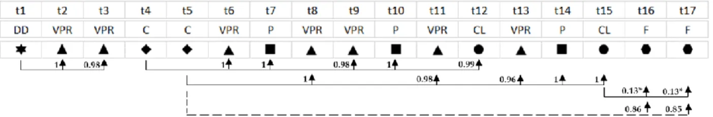
However, an indirect relation between C and F due to the cascade of three events, C→CL→F, is extracted as a direct relation by TPEX. These larger ranges are more representative for the range between the root cause and final consequence. In Fig. 3, the branching structure and the converged triggering probabilities for a subset of ss dataset is given as an illustrative example. These values are obtained by using second smallest discretization val-ues. The solid line shows instances of ground truth pat-terns and the values on the lines show triggering proba-bilities for the corresponding pairs. All of the pair in-stances except for those belonging to pattern CL→F have very high probabilities between 0.96 and 1. The probabil-ity of instances for the missed pattern is 0.13. These val-ues are eliminated during rank selection procedure due to the considerably higher probabilities calculated between root cause C and final consequence F which are 0.86 and .85 as a direct relation. The significance of the relation between C and F can decrease once the relation between the intermediate cause and final consequence is discov-ered by using appropriate discretization. For example, with smallest discretization we used, the probability be-tween C and F decreases to 0.4 whereas the probability of actual pairs CL→F increases from 0.13 to 0.6. This behav-ior is meaningful in the sense of conditional independ-ence. All the patterns TPEX found has high ranks as can be seen from the relatively darker areas in the rank map in Fig. 5. For the same discretization values, CSTP finds

TABLE1

EXPERIMENTAL DATA SETTINGS

λtriggering λtriggered Noise (%) Data Set _Name Average _{of N}

small small 0 ss 331 small small 5 ss5 310 small small 10 ss10 347 small medium 0 sm 439 small medium 5 sm5 520 small medium 10 sm10 457 small large 0 sl 691 small large 5 sl5 767 small large 10 sl10 783

small very large 0 svl 1123

small very large 5 svl5 1502

small very large 10 svl10 1385

large small 0 ls 562 large small 5 ls5 675 large small 10 ls10 692 large medium 0 lm 901 large medium 5 lm5 1023 large medium 10 lm10 1065 large large 0 ll 1286 large large 5 ll5 1488 large large 10 ll10 1585

large very large 0 lvl 2516

large very large 5 lvl5 2727

three of the five patterns in all datasets. The missing pat-terns are DD→VPR and C→VPR which have the longest interaction ranges in the data. The given neighborhood thresholds are greater than the distance between the events of these patterns, therefore, they can be captured based on the CPI threshold defined by the user. However, they are not in the top ten ranked patterns since their ranks change between 11 and 17. In other words, some irrelevant patterns are found more significant than these two patterns. As a result, they are shown with light colors in the rank map of CSTP. For the largest discretization, we observe 0.6, 0.8, and 1 for recall@10 with TPEX algo-rithm. All 0.6 values are observed for the datasets where the densities of the triggering events are large. CSTP achieves both 0.6 and 0.8 for recall@10 and there is no distinct pattern according to datasets.

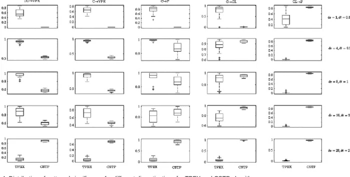
TPEX and CSTP measure the significance of a pattern using midmean and CPI, respectively. Fig. 4 shows their distributions for the ground truth patterns over 24

da-tasets by each discretization level. The patterns DD→VPR and C→VPR have considerably high significance values for TPEX than CSTP for all discretizations except for the roughest one. Although the use of a rough density func-tion significantly decreases the pattern probabilities calcu-lated by TPEX, it still achieves high ranks for them. For example, we can see from Fig. 5, DD→VPR is always ex-tracted within the top ten rank regardless of discretization level. It is even within the top five for most of the cases. The highest significance and rank values are obtained when the discretization is (s=8, t=1). CSTP usually yields 11 or 12 as rank of this pattern. TPEX shows simi-lar performance for the pattern C→VPR. There is a small decrease in probability and rank values for this pattern, but, it is still discovered within the top five for most of the cases. The ranks that CSTP produce, however, are usually greater than 13. Although CSTP has higher significance values for both patterns for the largest discretization, TPEX is still comparable based on the rank values. Simi-TABLE 2

RECALL@10:THE PERCENTAGE OFGROUND TRUTH PATTERNS FOUND WITHIN THE TOP TEN RANKED PATTERNS. Discretization

δs = 1, δt=0.05 δs = 4, δt=0.5 δs = 8, δt=1 δs = 16, δt=2 δs = 25, δt=25

Data Set TPEX CSTP TPEX CSTP TPEX CSTP TPEX CSTP TPEX CSTP

ss 0.8 0.2 0.8 0.6 0.8 0.6 0.8 0.6 0.8 0.8 ss5 0.8 0.2 0.8 0.6 0.8 0.6 0.8 0.6 0.8 0.8 ss10 1 0.2 0.8 0.6 0.8 0.6 0.8 0.6 0.8 0.8 sm 1 0.2 0.8 0.6 0.8 0.6 0.8 0.6 0.8 0.6 sm5 0.8 0.2 0.8 0.6 0.8 0.6 0.8 0.6 0.8 0.8 sm10 0.8 0.2 0.8 0.6 0.8 0.6 0.8 0.8 0.8 0.8 sl 1 0.2 0.8 0.6 0.8 0.6 0.8 0.6 0.8 0.6 sl5 0.8 0.2 0.8 0.6 0.8 0.6 0.8 0.6 1 0.8 sl10 1 0.2 0.8 0.6 0.8 0.6 0.8 0.6 0.8 0.8 svl 1 0.2 0.8 0.6 0.8 0.6 0.8 0.6 0.8 0.6 svl5 1 0.2 0.8 0.6 0.8 0.6 0.8 0.6 0.8 0.6 svl10 1 0.2 0.8 0.6 0.8 0.6 0.8 0.6 1 0.8 ls 1 0.2 0.8 0.6 0.8 0.6 0.8 0.6 0.8 0.8 ls5 1 0.2 0.8 0.6 0.8 0.6 0.8 0.6 0.6 0.6 ls10 1 0.2 0.8 0.6 0.8 0.6 0.8 0.6 0.6 0.6 lm 0.8 0.2 0.8 0.6 0.8 0.6 0.8 0.6 1 0.8 lm5 1 0.2 0.8 0.6 0.8 0.6 0.8 0.6 0.8 0.8 lm10 1 0.2 0.8 0.6 0.8 0.6 0.8 0.6 0.6 0.6 ll 0.8 0.2 0.8 0.6 0.8 0.6 0.8 0.6 0.8 0.8 ll5 1 0.2 0.8 0.6 0.8 0.6 0.8 0.6 0.8 0.8 ll10 1 0.2 0.8 0.6 0.8 0.6 0.8 0.6 0.8 0.6 lvl 1 0.2 0.8 0.6 0.8 0.6 0.8 0.6 1 0.8 lvl5 1 0.2 0.8 0.6 0.8 0.6 0.8 0.6 0.6 0.8 lvl10 1 0.2 0.8 0.6 0.8 0.6 0.8 0.6 0.8 0.6

Fig. 3. Example branching structure and triggering probabilities calculated by TPEX. Solid lines: true pairs, dotted lines: false pairs. The num-bers with asterisk show probabilities of pairs which are suppressed by the probabilities calculated for false pairs.

larly, TPEX is more succesful in discriminating the pat-tern C→P than CSTP for the first three discretization lev-els. For the discretization values (δs=16, δt=2) it is ob-served that TPEX produces higher significance values for the datasets where density of triggering events are small whereas CSTP has higher values when the density is large. Another observation is that for the ranks of the C→P, CSTP is affected by the noise. The more noise the data set has, the lower the rank of the pattern is. No such effect is observed for TPEX. CSTP is more successful in overall for the pattern C→CL. The success of TPEX in terms of high significance value depends on the discreti-zation levels. It extracts the pattern within the top five in

most of the cases, even though CSTP yields higher ranks for the same cases. Similarly, TPEX is able to find the pattern CL→F having the smallest interaction range if the smallest discretization is used. CSTP finds it with high significance.

We further examine the behavior of our algorithm for the pattern CL→F. We select the first nine datasets for further evaluation since the significance values calculated for these datasets are the worst which is 0.27 on average. In addition, the significance found for the indirect pattern C→F is 0.56, on the average, for the same set. We find two aspects that affect the performance in terms of accuracy. When we use even smaller discretization values for the Fig. 4. Distribution of patterns’ significance for different discretizations for TPEX and CSTP algorithms.

density function we observe an increase in the signifi-cance of CL→F from 0.27 to 0.36 and a decrease in the significance of C→F from 0.56 to 0.03. However, it also causes the significance of remaining true patterns to de-crease while keeping the ranks to be high. This is ex-pected, because we also claim in our findings that the significance of a pattern has its maximum if the discreti-zation is representative for the interaction range of the events the value of which can be obtained by D-function. Secondly, we observe that if the frequency of irrelevant data in the set is high, it affects the significance value of the pattern with considerably lower frequency negatively. In our scenario, we use small density values for the CL and F events to be representative for the real word situa-tions. However, in such settings, these events are repre-sented in the datasets with small frequencies relative to the other events such as VPR and P. Once we simulate the data with similar densities for all four event types, re-gardless of the discretization values used we achieve to find the pattern CL→F within the top ten ranked patterns and with a significance value around 0.2 while remaining patterns have high significance as well.

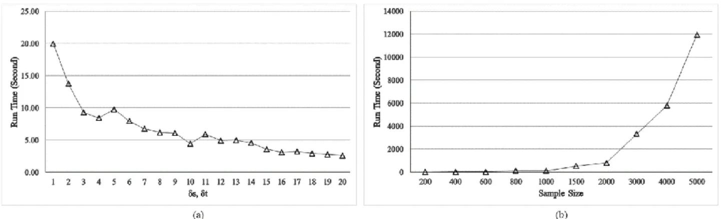
4.3 Computational Time and Complexity of TPEX In this paper, our focus is the predictive performance of the TPEX, however, we also evaluate its computational performance with respect to discretization level and the sample size. We used synthetic data sets with sample siz-es ranging from 200 to 5000. Data generation procedure is explained in detail in Section 4.1. To evaluate the effect of discretization level, we used discretization levels from 1 to 20. Fig. 6 (a) shows execution time of the algorithm in seconds with respect to discretization level. The range of each dimension of the synthetic data is 100. Therefore, the discretization values can be interpreted as percentage of the range of triggering function’s each dimension. For example, if t=2 then it means the time dimension of the density function consists of 50 bins each of which consti-tutes 2% of the range. We can see from the Fig. 6 (a), there is a fast decrease in execution time until t, s = 3 and then it decreases slowly as discretization level increases. Based on this results, using bin width which is smaller than 3% of the range increases execution time significant-ly. We examine the fluctuations around 5 and 10, and find that it is attributed to the number of iterations

re-quired to converge. For example, at t, s = 4 and t, s = 5 TPEX converges after 6 and 8 iterations, respectively. Thus, there is a decrease in execution time per iteration for t, s = 5.

The most influential factor on computational perfor-mance is the size of the dataset. Fig. 6 (b) shows execution time of the algorithm in seconds with respect to sample size. We observe sharp increase in the run time after N=2000. CSTP algorithm performs better than TPEX with respect to the computational time reported in [15].

The complexity of the algorithm is 𝑂(𝑘𝑛2 𝑇 𝑅

𝛿𝑡𝛿𝑠+ 𝑛

2_{+ 𝑛)}

where k is the number of iteration until convergence, n is the sample size, T is duration of time containing n events,

R is the study region, and t and s are discretization

pa-rameters for time and space dimensions of the triggering kernel, respectively. It is computationally expensive for the large data sets. The discretization parameters also add significant cost due to the high dimensionality of the pro-cess. Similar problems arise for the original baseline algo-rithm. Mohler et al. [21] propose to use a sampling proce-dure to reduce high computational cost arisen during the estimation step.

4.4 Sparsity

When the dimensionality and the number of bins are high and/or the number of observations is low, the estima-tions made by non-parametric methods might be nega-tively affected due to the small number of data samples falling into the bins resulting in a degree of sparsity. Stud-ies dealing with the sparsity issues in high dimensions can be found in the literature [29]. As long as the data points falling into the bins are accurate, the method will produce accurate estimations despite the limited number of data points. However real-world problems often in-clude noises which might yield unreliable estimation. Although dealing with the sparsity issue and selecting appropriate number of bins are beyond the scope of this paper, the approach we propose inherently is able to handle the problem to some degree. The data set size used to estimate the density functions is usually high by definition since the density function is defined by the pairwise distances instead of original sample size. In oth-er words, if thoth-ere is n numboth-er of obsoth-ervations, the density is estimated by (𝑛2_{− 𝑛)/2 + 𝑛 number of data points}

which is quite high. To demonstrate the sparsity problem, we choose the smallest data set we have experimented in this paper. In the case of ss data set in Table 2, the small-est sample size n is 205 within 10 replications. A total of 36 density functions for this data set is estimated by 21115 number of instances. In order to evaluate the reliability of the estimations with respect to discretization level, we made an extensive analysis by choosing this particular example in detail by considering both estimated pattern probabilities and their ranking. The results in Fig. 4 and Fig. 5 are presented based on the optimal discretization scale and its neighborhoods by considering all data points. For this particular example, on the other hand, we experimented the algorithm on a significantly large inter-val including extremely low and high discretization lev-els. Although discretization level affects the estimated probabilities of all possible patterns, their rank values change steadily. As we stated in Section 1, pattern proba-bilities are estimated with the highest probaproba-bilities if the discretization is made based on the interaction scales of the pattern which can be obtained by Diggle D function. For the other discretization values, these probabilities usually decrease. For example, in Fig. 7 (a), for the pat-terns DD→VPR and C→VPR, the estimated pattern prob-abilities are the highest where the discretization is made by s = 4 and t = 0.5 or s = 8 and t = 1 which are the most representative scales for the entire data. There is no significant change in probabilities for the neighboring discretization levels, however, their probabilities tend to decrease as they become distant from the optimum scale. In Fig. 7 (b), the ranks of the patterns are shown for dif-ferent discretization levels. The rank values decrease slowly compared to their probabilities. The most success-ful result is observed for the pattern C→CL. Its rank var-ies within the top five for most of the discretization levels.

The ranks of other patterns which interact within either longer or shorter distances are affected more as their dis-cretization become distant from the optimal scale. How-ever, they are observed within the top ten for most of the cases. This behavior is not observed for the random pat-terns. Besides having very small probabilities, they do not follow a rule with respect to discretization level. In fact they randomly fluctuate within a small probability range. In Fig. 7 (c) and Fig. 7 (d), for example, the reverse of the ground truth patterns are illustrated. Their behavior are random for both estimated probabilities and ranking. This example also shows that the proposed algorithm can reveal the causal structure in the data set successfully. The number of bins for space and time dimensions can be determined based on the results of Diggle D function which shows the extent of the space time interactions. They are determined by the parameters, t and s. These numbers determine the degree of the sparsity each densi-ty function has. If the parameters are too small, there will be many bins and the numbers of data points falling into them will decrease. As a result, pattern probabilities will be computed using few number of points present in a bin. If these data points have co-appeared on a scale by chance, then there is a high probability to calculate a higher rank of the corresponding pattern.

4.5 User Input Parameter Selection

TPEX requires users to define discretization values for the density function. There is no other threshold needed to be defined by users, for example, a threshold for the signifi-cance or neighborhood since it employs rank selection for the pattern extraction and the neighborhood is defined by the density function of distances. Note that a parametric density estimation procedure can also be employed in TPEX methodology. In such cases, discretization values are not needed to be defined, rather, a parameter estima-Fig. 7. (a) Estimated pattern probabilities for the ground truth patterns for different discretizations. (b) Ranking for the ground truth patterns for different discretizations. (c) Estimated pattern probabilities for the reverse of the ground truth patterns for different discretizations. (c) Ranking for the reverse of the ground truth patterns for different discretizations.

tion method such as MLE can be used in the algorithm. In such case where the form of the function is known, once the density is estimated, TPEX can be considered as a user input free algorithm for triggering pattern extraction. In the non-parametric case, the suitable discretization values can be obtained by using D-function if users are not sure about the appropriate values. On the other hand, if such values are not available, users may try different discreti-zation levels and evaluate them based on the calculated pattern probabilities which is maximum.

In the candidate generation approach, users are re-quired to define a neighborhood appropriate for the do-main as well as a threshold for the significance measure. A small neighborhood may cause missing patterns at global scales whereas larger ones may produce many ir-relevant patterns.

5

I

R

D

S

In the case study, we analyze whether the installation of speed bumps has reduced the number of accidents in the campus of Middle East Technical University (METU) be-tween 2002 and 2013. There is significant traffic flow in the center of the campus, especially at certain times of the day and on particular routes. To increase safety of pedes-trians, control the speed of the vehicles within the campus and reduce the number of traffic accidents, 41 speed bumps were built in different years ranging from 1999 to 2011 on the roads where pedestrians are dense and driv-ers tend to speed up, in addition to the speed limit al-ready applied in the campus.

We select the campus as a study region due to several factors: (1) We have an access to domain knowledge to assess the ability of our proposed approach (2) Although traffic is a complex problem, this particular region has limited number of unknown or uncontrollable factors unlike the city centers where there might be several fac-tors for accidents. (3) The date of installations of speed bumps, the reasons and dates of the accidents are record-ed and available.

5.1 Data Set

We considered the accidents related to pedestrian, and vehicle crashes which are fully and promptly reported but we excluded the accidents caused by external factors. For example about half of the reported accidents occur at the gates of METU due to hitting cars to the malfunction-ing gate barriers. As a result, our data set comprises 64 in-campus accidents.

The data set has been prepared for the analysis as fol-lows: The approximate geographic locations of the acci-dents are identified from the explanations in the reports and their coordinates are determined by using Google Earth. Representing a speed bump as a spatio-temporal event require further data processing. A speed bump co-vers an area instead of a single point in space. In addition, its existence in time is a duration once it is constructed. Therefore, some transformation is needed to represent each speed bump as a spatio-temporal point data. The spatial location can be expressed by a representative point

such as center. On the other hand, their existence in time is only relevant during the time of the accidents. As a re-sult, temporal dimension has been defined based on the time snapshot of each accident.

Generating a speed bump map of the campus for each accident results in 3968 (64x62(due to speed bumps counted twice for two way roads)) speed bumps in total. This class imbalance usually cause difficulties during the modeling. For example, the pairs between the types relat-ed with sperelat-ed bumps such as (exist, exist), (exist, non-exist) and (non-exist, non-non-exist) have signicantly higher frequency than the pairs such as (exist-accident) and (non-exist-accident) in the data. Therefore, resampling has been carried out. In addition, the pairs between the types related with speed bumps may show spatio-temporal clusters since there are usually more than one speed bump within a small region. As a result, those pairs are expected to be extracted, and due to the null addition effect, they may suppress the significance of those con-taining accidents.

It has been observed by the domain experts that the deceleration starts at around 100 meters before the speed bumps and their speed prevention effects disappear around 100-150 meters after them in the campus. As a result, we have selected speed bumps within 150 meters neighbourhood of the accidents which yield 137 resampled data. In order to encode event types related to the speed bumps, we consider three situations: In the neighborhood of some of the accidents (ACC) (1) there are one or more speed bumps (SB) (2) one or more speed bumps are built before the most current accident ob-served (NSBY: No Speed Bump Yet) (3) there is no speed bump and there will not be any in the future (NSB: No Speed Bump).

5.2 Results and Discussions

In order to evaluate the effectiveness of our approach we use the following evaluation scheme. There are 16 possible patterns out of which the rank and probabilities of NSBY→ACC, NSB→ACC and SB→ACC need to be assessed in order to investigate the impact of the speed bump installations on number of accidents. Assesment of the results in this case study differs slightly from the sim-ulated scenario in terms of pattern probabilities. In the simulation data sets, the ground-truth patterns are inde-pendent from each other whereas in this real case 3 ex-pected patterns are related. According to the METU traf-fic oftraf-ficers we consulted, speed bumps were reported as they have decreased the number of accidents inside the campus. It means that the probability of patterns includ-ing NSBY→ACC, NSB→ACC are expected be higher than the pattern probability of SB→ACC. Table 3 shows the top five ranked patterns and their probabilities obtained by our proposed approach TPEX and CSTP. In the table, δs = 160, δt = 10 is the discretization level suggested by Diggle D-function. We also examine the results for small-er and largsmall-er discretization levels. The values in the parantheses show the support count of the patterns. The results indicate that TPEX finds the expected three pat-terns at the top three for the optimal discretization level

and at the top four for the smaller. For the highest level, TPEX does not find any pattern. In other words, the events are random or not related at that scale according to our proposed approach. On the other hand, CSTP finds these patterns at the top three for the first and second lowest discretization levels. However, it underperforms when the discretization level becomes higher. Irrelevant patterns such as SB→SB appear at the top three. This is due to the fact that larger neighborhood decrease the pre-cision by allowing distant pair instances be related.

In these type of problems, sequential pattern mining algorithms usually apply a pre-filtering based on support count to remove insignificant or irrelevant patterns and a cut-off support value can be found in favor of both ap-proaches. NSBNSBY pattern with one support count can be considered as a noise and discarded from the results of TPEX. Similarly, depending on the support threshold, SBSB pattern with nine support count can be filtered out from the results of CSTP.

In this particular case study, attention should be paid to the probabilities of the patterns extracted by both algo-rithms. According to the TPEX results, absence of speed bumps (NSBACC, 0.999(33); NSBYACC, 0.889(17)) are more likely to trigger accidents than presence of them (SBACC, 0.647(32)). In CSTP, the probability of the pat-terns (SBACC, 0.328(32)) and (NSBYACC, 0.219(17)) are conflicting such that the installation of speed bumps appeared to trigger more accidents compared to the pre-vious cases where there are no speed bumps. As there are still other causes for traffic accidents such as violation of traffic rules and speed, SB→ACC pattern is expected to be extracted by the algorithms.

6

C

A spatio-temporal event can be an observed disease, the location where a forest fire has started, a crime committed at a location, a traffic accident, and so on. Exploring rela-tionships within and among types can provide valuable

information for several domains such as public safety, crime prevention, epidemiology and environmental stud-ies. We proposed a new methodology to solve sequential pattern mining problem which is usually handled by fre-quency based candidate generation approaches. Our methodology operates on continuous spatio-temporal domain. Specifically, our focus is spatio-temporal se-quences whose elements are related according to an un-known triggering or branching structure. The algorithm can be successfully implemented in various domains, es-pecially for the domain for which the underlying behav-ior is not known. Traditional frequency based approaches and the constant neighborhood thresholds commonly used in the sequential mining literature are not capable of explaining such complex and unknown relationships. Therefore, in order to capture this challenge, we reformu-lated the sequential pattern mining problem in this study. We defined the problem with conditional probabilities and provided estimation procedure for the conditional intensity model which uses multivariate Hawkes model in the MISD algorithm.

Our results show that TPEX is able to find patterns that exist in the data with high ranks. Significance of a pattern increases as discretization values of triggering functions are getting closer to the significant interaction ranges suggested by Diggle D. We use midmean of the pairwise probabilities of instances, which constitute a pattern as the significance measure of the pattern. The measure is successful in discriminating true patterns. It usually as-signs high probabilities for the true patterns while it is able to remove irrelevant patterns by estimating their sig-nificance close to 0. The sigsig-nificance measure we pro-posed is variant under the null addition operation if the frequency of the elements of a pattern significantly low relative to the irrelevant event types. In most of the real situations, there may be patterns in the data at different scales. TPEX can give information about the true interac-tion scale of a pattern due to its relainterac-tion to Diggle-D. In TABLE 3

TOP FIVE RANKED PATTERNS AND THEIR PROBABILITIES EXTRACTED BY TPEX AND CSTP.PP AND SC STAND FOR PATTERN PROBABILITY AND SUPPORT COUNT RESPECTIVELY

Discretization

TPEX δs = 40, δt=2.5 δs = 80, δt=5 δs = 160, δt=10 δs = 320, δt=20

Rank Pattern PP/SC Pattern Pattern _Prob. Pattern Pattern _Prob. Pattern Pattern _Prob.

1 NSBACC 1(28) NSBACC 1(29) NSBACC 0.999(33) - -

2 NSBNSBY 1(1) NSBNSBY 1(1) NSBYACC 0.889(17) - -

3 NSBYACC 0.965(15) SBACC 0.785(29) SBACC 0.647(32) - - 4 SBACC 0.739(29) NSBYACC 0.783(20) SBNSBY 0.507(11) - - 5 SBNSBY 0.214(41) NSBYNSBY 0.499(8) NSBYNSBY 0.434(12) - -

CSTP δs = 40, δt=2.5 δs = 80, δt=5 δs = 160, δt=10 δs = 320, δt=20

Rank Pattern PP/SC Pattern Pattern _Prob. Pattern Pattern _Prob. Pattern Pattern _Prob.

1 NSBACC 0.203(13) NSBACC 0.344(23) NSBACC 0.422(29) NSBACC 0.422(29) 2 SBACC 0.156(10) SBACC 0.281(22) SBACC 0.328(32) SBACC 0.328(34) 3 NSBYACC 0.063(4) NSBYACC 0.141(11) SBSB 0.267(9) SBSB 0.300(11) 4 ACCACC 0.016(1) ACCACC 0.031(2) NSBYACC 0.219(17) NSBYACC 0.219(17) 5 - - ACCNSBY 0.016(1) NSBYNSBY 0.125(2) NSBYNSBY 0.188(3)