Design of Fuzzy Logic Controller for a PV Grid Connected Two Area Load Frequency Control System

(1)

---*---Abstract -**

In this paper, a PV grid connected two-area load frequency control system with 45% penetration level is presented. The model of the two-area system is introduced and the system frequency errors due to various cases of load changes are studied in this PV connected power grid. The design of appropriate and effective fuzzy logic controller (FLC) is presented to regulate those errors to keep the system response within the required specifications: settling time less than 3s, undershoot less than 0.02 Hz and steady state error equal to zero. The system response due to FLC is also compared to that due to the conventional PI controller designed for the same system.

Key Words: Fuzzy control, load frequency control, PV.

1.INTRODUCTION

As the contribution of renewable energy is becoming an essential part of the power generation, it is of critical importance to study the effects of this increased penetration of the renewable energy resources on the power system and study the potential problems associated with it. The load frequency control (LFC) is one of the main points to be considered in the study of this interconnected system. [1] In this paper, a well-structured fuzzy logic controller (FLC) has been designed to assure a continuous and steady system performance through system frequency control.

In this paper, section 2 presents the model of the two-area LFC connected to PV system. Section 3 explains the FLC design details and the response of the system with the FLC implemented. Section 4 shows the comparison between the response of the uncontrolled system and the controlled system. Also, it presents the comparison between the responses for the system with the conventional PI controller only, and that with FLC included.

2.MODEL OF THE TWO-AREA LFC

The general components of the LFC are: The governor which is used to monitor and measure the system speed changes and to control the valve. The turbine which is the component that transforms the input energy (in this case coming from the steam) into mechanical energy that could then be an

input to the generator which will transform this mechanical energy into electrical energy. The reheater makes the system more efficient as it reheats the steam to keep the same high temperature of the steam that entered the governor. [2] In this section the specific mathematical model of each area has been presented along with the connection of these two areas in one system and the response of this system without controllers. The final model is shown with the photovoltaic system connected to it. This PV system has been designed separately based on [ 3] but is not the focus of this paper. The integral controller is required in both areas since one of the criteria to be met is a steady state error equal to zero. Since the integral controller adds one state variable to the model of the system, it has been included to the models of both areas for which the FL controller is designed.

2.1Mathematical Model of Area 1

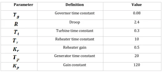
[image:1.595.302.566.475.593.2]

The state model of the first area in this LFC with only the integral controller is presented here. Table 1 shows the parameters that were used in the modeling of the thermal LFC under study and their definition.

Table -1:Parameters of the thermal power system

Parameter Definition Value

Governor time constant 0.08

Droop 2.4

Turbine time constant 0.3

Reheater time constant 10

Reheater gain 0.5

Generator time constant 20

Gain constant 120

Figure 1 shows the block diagram representation of this area. The change in load power is the input to this area which is considered to be a disturbance.

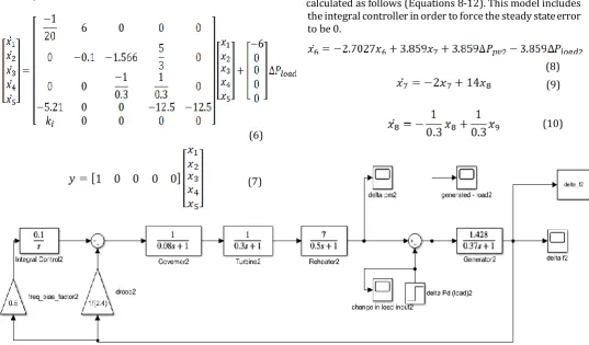
The following state equations (Equations 1-5) represent area 1. As explained earlier, adding an integral controller to the system increases the number of state variables by 1, thus, the system now has a total of 5 state variables instead of only 4. An integral controller with the gain value Ki =0.6 produced

(2)

with an integral controller becomes the following (Matrices 6 and 7).

[image:2.595.29.572.44.416.2]

2.2 Model of the Second Area

Table -2: Parameters of area 2 model.

Parameter Definition Value

Governor time constant 0.08

Droop 2.4

Turbine time constant 0.3 Reheater time constant 0.5

Reheater gain 7

Generator time constant 0.37

Gain constant 1.428

Table 2 shows the parameter from which the state model of area 2 has been constructed and Figure 2 shows the block diagram. The state space equations of this LFC have been calculated as follows (Equations 8-12). This model includes the integral controller in order to force the steady state error to be 0.

(1)

(2)

Fig -1: Block diagram of area 1.

(3)

(4)

(5)

(6)

[image:2.595.308.566.266.389.2]

(7)

Fig -2: Block diagram of area 2 in the LFC power system.

(8) (9)

[image:2.595.29.567.434.749.2]

(3)

For the connection of these areas together, there are 5 state variables from the first area and 5 state variables from the second. However, the interconnection adds one more state variable because of the tie-line power change giving a total of 11. For each area there is the input of change of load power and another input from the PV system connected to the grid. Therefore, for this interconnected system, it has 4 inputs

( , , & ) and 2 outputs which are

the change in frequency of area 1 ( ) represented by the 1st

state variable and the change in frequency of area 2 ( )

represented by the 6th_{state variable.}

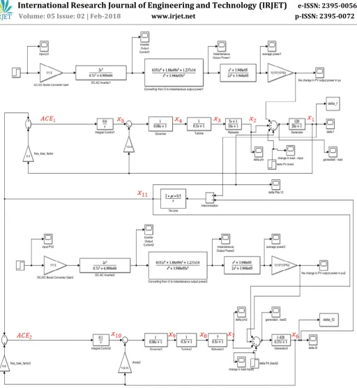
As to the full model of the two-area LFC system, it is obtained by combining Equations 1-5 and 8-12 along with the following modifications (demonstrated in Equations 15-18) which give the state model accounting for the interconnected parts between both areas. The state model of the two-area

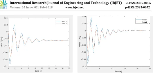
system connected to PV is shown in matrices 19-22. The controllability and observability of the system have also _{been checked and the two-area system is controllable and} observable. The stability of the system has also been verified. Figure 3 shows the response of the two-area system without any controller (without even the integral controller), Figure 4 and Figure 5 show the response of both outputs in this system with integral controller for various changes in load (reasonable change in load and an extreme change in load (50%)). Figure 7 shows the block diagram of the interconnected two-area system with PV with integral controllers.

(13)

(14)

(19)

(20)

(21)

(22)

(15)

(16)

(4)

[image:4.595.38.566.46.300.2]

[image:4.595.298.563.53.298.2]

controller due to 50% increase in load.

Fig -4: Change of frequency of both areas (for the system with integral controller only) for reasonable load.

It is observed that without using the integral controller the steady state frequency error does not disappear, which is undesirable. When including the integral controller, the steady state error requirement is met, however the settling time is much larger than the required 3s (it is more than 18s in both cases) and the undershoot is also much larger than the required 0.02 Hz. The second case of a sudden increase in load equal to 50% is an extreme case. However, even in the first case (i.e. reasonable change in load power), neither the undershoot nor the settling time criteria were met with integral controller only. Thus, FL controller is designed to enhance the system performance in terms of system frequency.

Fig-5: Change of frequency of both areas (for the system with integral controller only) for 50% increase in

load.

3.FUZZY LOGIC CONTROLLER DESIGN

The concept of fuzzy logic [4] is based on a concept similar to that of the binary logic (0,1). However, in the binary logic, any value can either be in a set (therefore, having a value of 1) or not in a set (having a value of 0). Things in the binary logic are either black or white. But in fuzzy logic, each value can be considered as a member of a set by a certain percentage (either a low or a high percentage). Thus, the values in fuzzy logic have partial memberships in the set. [5]

Figure 6 shows the general steps of designing a fuzzy logic controller (FLC) for a system. After defining the input(s) of the FLC, membership functions and the ranges corresponding to each should be determined through the stage called Fuzzification. The number of these membership functions and what each one represents are determined.

[image:4.595.41.290.347.541.2] [image:4.595.301.566.570.635.2]

(5)

square of the number of membership functions chosen. The output of the fuzzy logic controller is obtained based on these rule as a fuzzy value, then the last stage (Defuzzification) occurs to transform it from a fuzzy value to a numerical value. The most commonly used defuzzification method is the Centre-of-Gravity (Centroid) by weighing all the membership functions for all variables (by weighing the control actions). [5]

In the system presented in this paper, two inputs were chosen for the fuzzy logic controller; the system frequency

error and the derivative of the error. [6]. In control systems, usually the error derivative is chosen as a second input to the FL controller because the derivative of a curve is the slope, which indicates the direction of the curve at each point. This is crucial in determining what the controller output should be based on whether the error is decreasing or increasing at that point. [5]

[image:5.595.46.559.48.605.2]

The range of both these inputs should cover all the possible values of the error and the change in error. Thus, the ranges of error and change in error have been checked for various loads, and the values never exceeded -3 and 3. Thus, this is the range chosen for both.

Fig -7: Block Diagram of the two-area system connected with the PV system.

(6)

it is negatively feedback to the system. The range of this output has been chosen to be -0.5 and 0.5. This is the range that produced the best response.

As to the first stage of fuzzy logic controller design which is the fuzzification, the membership functions chosen are 7. First, 3 and 5 membership functions were tried but did not give the required specifications. Also, 9 membership functions have been studied but did not have any noticeable enhancement on the response than with only 7 membership functions. Therefore, the best number for this application was 7 and they are the following: Negative Big (NB), Negative Medium (NM), Negative Small (NS), ZZ (Zero Change), Positive Small (PS), Positive Medium (PM) and Positive Big (PB).

Ranges of membership functions have been distributed equally among all membership functions from the original range (between -3 and 3 for the inputs and -0.5 to 0.5 for the output). Narrower ranges at some points are only required when fine tuning and very accurate control is necessary at a certain small range. [5] For the current application, narrower ranges were tried but did not give much difference. Thus, the equal ranges were implemented. As to the shape of these functions, triangular shape was chosen.

The next stage in the design is creating the rules from which the inference procedure will take place. Table 3 shows the rules designed in this work and that gave the best response for the system.

Table -3:Rules designed for this FL controller

NB NM NS ZZ PS PM PB

NB NB NB NB NB NS NS ZZ

NM NB NM NM NM NS ZZ PS

NS NB NB NM NS PS PM PB

ZZ NB NM NS ZZ PS PM PB

PS NM NS ZZ PS PS PM PM

PM NS ZZ PS PM PM PM PM

PB ZZ PS PM PB PB PB PB

The last stage in the fuzzy controller design is defuzzification, i.e. changing the fuzzy value of the controller output into a numerical value that could be feedback to the system. There are several methods for defuzzification and the one applied in this controller is the centroid (center of gravity) method as it is the most commonly used.

An example of the defuzzification method is applied here to illustrate the concept. Assume at one point the error has a value of -3, this means that we are 100% certain that the error is NB at this point according to the triangular shapes of the membership functions. Thus, it has a membership value of 1. Assume at the same point that the derivative of the

error is -2.5. This means we are 50% certain that it is NB and 50% certain that it NM. This produces two possible rules to be applied:

ul s N n s N t n u ontroll r output is NB

ul s N n s NM t n u ontroll r output is NB

Applying the inference method of minimum for both these rules:

Thus, both rules have a probability of 0.5. They are equally likely in this example. To do the defuzzification based on weighing each rule, the center of NB is -3, and the center of NM is -2. Calculating the shaded area of the triangle for the derivative of the error:

According to these values, the controller output can be calculated [7] as in Equation 25:

Negative Big value which is why the output is NB. The exact value of the output would be the value that matches -2.5 on the output scale which is (-0.5 and 0.5). By calculation, this value would be:

[image:6.595.307.545.353.417.2]

By checking the output on MATLAB for the same input values using, the value obtained was almost the same (-0.43). Figure 8 shows the block diagram of the PV grid connected two-area LFC system with this FL controller applied and with PI controller. The Kp and Ki values in the PI controller of

area 1 were modified to Kp =0.6 and Ki =0.9 and for the

second area Ki =1.1 because they gave the best response in

the two-area system.

(23)

(25)

(7)

to a reasonable change in load that is equal between both systems. The tie-line power change between both areas is shown in Figure 11. For this case, the response is within the required criteria for the undershoot, the settling time and the steady state error. The settling time is close to the required range due to the limitation of the fuzzy logic

[image:7.595.27.567.43.666.2]

(8)

[image:8.595.22.291.134.312.2]

with PI controllers and to the uncontrolled system.

[image:8.595.307.562.210.387.2]

Fig. -9: Response of area 1 with PI and fuzzy logic controllers for equal and reasonable change in load.

[image:8.595.20.292.355.533.2]

Fig -10:Response of area 2 with PI and fuzzy logic controllers for equal and reasonable change in load.

Fig. -11: Tie-line power change between area 1 and 2 for the system with PI and FLC (reasonable change in load).

Figure 12 and Figure 13 show the response of the two-area system with a sudden 50% increase in load. Figure 14 shows the tie-line power change between both areas for this case. The criteria of undershoot and settling time are not exactly met, but they are fairly acceptable since this is the assumed worst-case scenario. A big improvement of the system response can still be observed from the uncontrolled case or the controlled with PI.

Fig. -12: Response of area 1 with PI and fuzzy logic controllers for 50% change in load.

[image:8.595.22.301.584.739.2]

(9)

[image:9.595.249.569.49.259.2]

the system with PI and FLC (50% change in load).

4.RESULTS AND COMPARISON ANALYSIS

PI controller has been designed for the same system. When applying only the conventional PI controller to the LFC system described in this paper, the system had more oscillations and worse undershoot and settling time as shown in Figures 15 and 16. It did improve the system compared to the response of the uncontrolled system, however, even with the optimized values of and obtained in this work, neither the settling time nor the undershoot specifications were met. Therefore, advanced controllers such as FLC were required.

[image:9.595.26.381.51.247.2]

It can be observed in the two-area LFC system that FLC improved the frequency oscillations and undershoot greatly compared to the system with the conventional controller (PI) only. Moreover, FLC made the response of the system satisfy all conditions (as to the settling time, it is close to the required value (3s)). This shows one of the biggest advantages of FLC which is the ability to force the system to meet the specifications even when the model of the system becomes very complicated. [8] As to the extreme case of 50% increase in load, FLC did not satisfy the undershoot requirement. However, this is the worst-case scenario and the FL controller still makes a big enhancement.

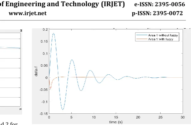
[image:9.595.309.571.310.500.2]

Figure 15 and Figure 16 show a comparison between the responses of area 1 and 2 with the PI controller and with FLC to observe this enhancement. In addition, Table 4 summarizes the specification values for all cases: uncontrolled and controlled (with reasonable change in load and extreme change in load).

Fig. -15: Comparison between two-area system response with PI and FLC (area 1) due to 50% increase in load.

Fig. -16: Comparison between two-area system response with PI and FLC (area 2) due to 50% increase in load.

Table -4: Comparison between the response specifications for the uncontrolled system and due to PI

and FLC

Settling Time Undershoot Steady State Error Area

1 Area 2 Area 1 Area 2 Area 1 Area 2

Case 1

(reason-able increase

in load)

PI 9.598 22.1 -0.033 -0.018 0 0

FLC 7.4 6.48 -0.017 -0.014 0 0

Case 2 (50% increase

in load)

Uncontrolled 23.14 20.6 -0.087 -0.067 -0.03 -0.03

I 15.11 14.1 -0.093 -0.071 0 0

PI 9.598 22.1 -0.083 -0.045 0 0

[image:9.595.303.567.598.746.2]

(10)

This paper presented a model for a two-area LFC system connected to a PV system. Fuzzy logic controller has been designed and applied to this system in order to control the frequency of the system due to various load changes. It has been observed that the conventional PI controller was not sufficient to meet the required specifications for the system frequency (undershoot less than 0.02Hz, settling time less than 3s and steady state error equal to zero). Therefore, FLC was essential to enhance the performance of the system. FLC made the undershoot and the steady state error meet the criteria and made the settling time close to the required value. This shows the big advantage of FLC in that it enhances the system performance regardless of the complexity of the mathematical model of the system. Thus, even with systems that have complex mathematical models, a much-enhanced response can be achieved using FLC.

ACKNOWLEDGEMENT

The authors wish to thank RIT Dubai for the support.

REFERENCES

[1] A. Ik , A. Kulk rn , D. V r s , “Lo r qu n ontrol

using fuzzy logic controller of two-area thermal-thermal power plant,” Int rn t on l Journ l o Em rg ng Technology and Advanced Engineering, ISSN 2250-2459, vol. 2, issue 10, October 2012.

[2] A. Mont n F. Pon , “El tr pow r s st ms”,

Intelligent Monitoring, Control, and Security of Critical

Infrastructure Systems Springer, 2015. DOI

10.1007/978-3-662-44160-2_2)

[4] M. C v utt , “Fu g n s ul ng,” Control

Engineering Laboratory, Helsinki University of Technology, Sci Rep. 62, 2000.

[5] G. Chen and T. Pham, Introduction to Fuzzy Sets, Fuzzy

Logic, and Fuzzy Control Systems, New York: CRC Press LLC 2001.

[6] P. D bur, N. Y v n . Avt r, “MATLA D s gn n

Simulation of AGC and AVR For Single Area Power System with Fuzzy Logic Control.,” Int rn t on l Journ l of Soft Computing and Engineering (IJSCE), ISSN: 2231-2307, vol. 1, Issue-6, January 2012.

[7] K.M. Passino, S. Yurkovich, Fuzzy Control, California:

Addison-Wesley, 1998.

[8] J. Go j v , “Comp r son b tw n PID n u

ontrol,” Dép rt m nt ’In orm t qu , E ol

Polytechnique Fédérale de Lausanne, Switzerland.

BIOGRAPHIES

Samar A. Emara Born in

1994. Graduated with BSc in Electrical Engineering from the Petroleum Institute, Abu Dhabi in 2016. Currently doing MSc in Electrical

Engineering (in control

systems) at RIT Dubai. Worked as a teaching assistant for the academic year (2016-2017) at RIT Dubai and is currently a full time Master student. Samar is a student member of IEEE and has filed a patent of the project entitled (Design of Nanomagnetic Tagging and Monitoring System) in 2016.

Abdulla Ismail Professor of

Electrical Engineering. Emirati citizen, Born in Sharjah. BSc (‘80), MS (’83), n P D (’86) in Electrical Engineering from University of Arizona, USA. 1st Emirati to hold a PhD in Engineering. Has over 30 years

Coauthored two books; desalination technology in the UAE and Contemporary Scientific Issues. Published over 90 referred technical papers in local and international journals and conferences. Won Emirates Energy Award (Education and Energy Management), 2015. Won several UAEU awards for University and Community service. Won the Fulbright scholarship, USA Government. A senior member of IEEE.

A member of Dubai KHDA University Quality Assurance International Board, Chair of the Zayed Future Energy Prize (Global High Schools Committee), Chairman of AURAK Engineering Advisory Council.

[3] M. Al m n F. K n, “Tr ns r un t on m pp ng or grid connected PV system using reverse synthesis t n qu ,” n 4t Works op on Control n Mo l ng for Power Electronics (COMPEL)-IEEE, 2013.

of teaching and research experience at UAE University (ALAIN) and RIT Dubai.

Design of Fuzzy Logic Controller for a PV Grid Connected Two Area Load Frequency Control System

---***---Abstract -

---*---Abstract -**