A Review of Measurement Integrated Simulation of Complex Real Flows

http://dx.doi.org/10.4236/jfcmv.2015.32006

A Review of Measurement-Integrated

Simulation of Complex Real Flows

Toshiyuki Hayase

Institute of Fluid Science, Tohoku University, Sendai, Japan Email: [email protected]

Received 21 November 2014; accepted 16 February 2015; published 3 April 2015

Copyright © 2015 by author and Scientific Research Publishing Inc.

This work is licensed under the Creative Commons Attribution International License (CC BY). http://creativecommons.org/licenses/by/4.0/

Abstract

In spite of the inherent difficulty, reproducing the exact structure of real flows is a critically im-portant issue in many fields, such as weather forecasting or feedback flow control. In order to ob-tain information on real flows, extensive studies have been carried out on methodology to inte-grate measurement and simulation, for example, the four-dimensional variational data assimila-tion method (4D-Var) or the state estimator such as the Kalman filter or the state observer. Mea-surement-integrated (MI) simulation is a state observer in which a computational fluid dynamics (CFD) scheme is used as a mathematical model of the physical system instead of a small dimen-sional linear dynamical system usually used in state observers. A large dimendimen-sional nonlinear CFD model makes it possible to accurately reproduce real flows for properly designed feedback signals. This review article surveys the theoretical formulations and applications of MI simulation. For-mulations of MI simulation are presented, including governing equations of a flow field observer, those of a linearized error dynamics describing the convergence of the observer, and stabilization of the numerical scheme, which is important in implementation of MI simulation. Applications of MI simulation are presented ranging from fundamental turbulent flows in pipes and Karman vor-tices in a wind tunnel to clinical application in diagnosis of blood flows in a human body.

Keywords

Real Flow Field, State Observer, Numerical Simulation, Measurement, Measurement-Integrated Simulation

1. Introduction

solution that reproduces the exact instantaneous structure of the real flow such as a turbulent flow, but rather one having the same statistical characteristics as those of the relevant flow [1]. It is quite difficult to obtain the exact flow solution because: 1) it is difficult to specify the initial and/or boundary conditions of real flows correctly; and 2) even if these data are available, a small error in the initial condition will increase exponentially in struc-turally unstable dynamical systems such as turbulent flows [2].

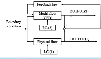
In spite of the inherent difficulty, reproducing the exact structure of real flows is a critically important issue in many fields, such as weather forecasting or feedback flow control. In numerical simulation used for weather fo-recasting, the initial condition is updated at time intervals based on past computational results and measurement data around the computational grid points. In meteorology, extensive studies have been carried out on such me-thods, which are termed data assimilation [3]. The four-dimensional variational method (4D-Var) is widely used in numerical weather forecasting [4]-[6], but it requires huge computational power to repeatedly solve flow dy-namics and its adjoint, and, therefore, is not suitable for application to problems of real-time flow reproduction such as feedback flow control. A similar concept, namely, interactive computational-experimental methodology (ICEME), was proposed by Humphrey [7] for application to engineering problems, in which the measurement data are supplied to a thermal-flow simulation to enhance the efficiency of computation. Possible advantages of ICEME as well as further necessary studies were discussed in relation to a complex flow-related optimization problem seeking the optimum arrangement of electrical heat sources to minimize the temperature in a ventilated box under some constraints. Zeldin and Meade [8] applied the Tikhonov regularization method, which is com-mon in inverse problems, to obtain an optimum solution for estimation of the real flow from the numerical and measurement results of the relevant flow. Particle imaging velocimetry (PIV) has proved to be a mature method to obtain velocity vectors in a flow domain. Studies have been made on the application of CFD schemes to mod-ify PIV measurement so as to satisfy physical constraints such as the continuity equation [9]. State observer, which is a fundamental methodology in modern control theory to estimate the state variables from the state equ-ation with the aid of partial measurement data, has been used in flow problems. Uchiyama and Hakomori [10] reproduced the unsteady flow field in a pipe using a Kalman filter, which is a special state observer [11]. Högberg et al. [12] constructed a Kalman filter to estimate the flow state from the information on the wall in a numerical experiment for the optimum control of the subcritical instability of a channel flow based on a linea-rized equation. The Kalman filter and state observer seek the asymptotic convergence to the optimum state re-quiring only one forward integration from an arbitrary initial condition. Having much less computational load, they are potential candidates to solve the problem of how to reproduce real flows. Comparison of the Kalman filter and state observer shows that the latter has a simpler structure and retains an essential part of the state es-timation. The present author [13] proposed a measurement-integrated simulation (hereafter abbreviated as “MI simulation”), which is a kind of observer using a CFD scheme as the mathematical model of a relevant system, and successfully applied it to a turbulent flow in a square duct, a Karman vortex street behind a square cylinder [14] [15], and blood flow in an aneurismal aorta [16].

Figure 1. Block diagram of measurement-integrated (MI) simulation.

other existing observers, is the usage of a CFD scheme as a mathematical model of the physical flow. A large dimensional nonlinear CFD model makes it difficult to design the feedback law in a theoretical manner; there-fore, it has been determined by a trial-and-error method based on physical considerations. However, it makes it possible to accurately reproduce real flows once the feedback law is properly designed.

This review article deals with the theoretical background and applications of MI simulation. In Section 2, formulations of MI simulation are presented, including governing equations of an observer for a flow field, those of a linearized error dynamics describing the convergence of the observer [21], and stabilization of the numerical scheme, which is important in implementation of MI simulation [22]. Applications of MI simulation presented in Section 3 range from fundamental turbulent pipe flows [1] [13] [23] and Karman vortices in a wind tunnel [14] [24] to clinical application to diagnosis of blood flows in a human body [16] [25]-[27].

2. Formulation of Measurement Integrated Simulation

2.1. Governing Equations

Measurement-integrated simulation deals with incompressible and viscous fluid flow. The dynamic behavior of the flow field is governed by the Navier-Stokes equation:

(

)

p

t ν

∂ _{= − ⋅∇ + ⋅ ∆ − ∇ +}

∂

u

u u u f (1)

and the equation of mass continuity:

0

∇ =u (2) as well as by the initial and boundary conditions. In the Navier-Stokes Equation (1), p denotes the pressure di-vided by density, and f denotes the body force didi-vided by density which is defined as the feedback signal in the MI simulation. The pressure equation is derived from Equation (1) and (2) as

(

)

{

}

div .

p

∆ = − u⋅∇ u + ∇f (3)

We use Equations (1) and (3) as the fundamental equations.

The basic equation of the MI simulation is represented as a spatially discretized form of governing equations (1) and (3):

( )

( )

T

d

d ,

N

N N N N N N N N N N N

t

 _{= − ∇ +}

 

∆ = + ∇



u

g u p f

p q u f

(4)

where uN and pN are computational results for the 3N-dimensional velocity vector and the N-dimensional

pres-sure vector, respectively, N denotes the number of grid points, gN, qN, ∇N and ΔN are matrices which express the

discrete form of operators g, q, ∇, and Δ. The operators, g and q are defined as follows

( )

(

)

( )

{

(

)

}

.

div

q

ν

 = − ⋅∇ + ⋅ ∆ 



= − ⋅∇



g u u u u

u u u (5)

OUTPUT(2) Feedback law

Model flow (CFD)

I.C.(2)

Physical flow

I.C.(1)

OUTPUT(1) Boundary

condition

OUTPUT(2) Feedback law

Model flow (CFD)

I.C.(2)

Physical flow

I.C.(1)

OUTPUT(1) Boundary

condition +

ｰ

OUTPUT(2) Feedback law

Model flow (CFD)

I.C.(2)

Physical flow

I.C.(1)

OUTPUT(1) Boundary

condition

OUTPUT(2) Feedback law

Model flow (CFD)

I.C.(2)

Physical flow

I.C.(1)

OUTPUT(1) Boundary

condition +

[image:3.595.211.419.82.205.2]

It is noted that effects of the boundary conditions are included in the functions gN and qN.

We define the operator D_N

( )

• to generate the N-dimensional vector consisting of the values of a scalar field sampled at N grid points. The definition of DN is naturally extended to the case when the variable is a velocity

vector field as D_N

( )

u = D_N

( )

u₁ T D_N

( )

u₂ T D_N

( )

u₃ T_T. Applying the operator to the Navier Stokes equa-tion and the pressure equaequa-tion, we obtain the sampling of these equaequa-tions at N grid points.

On the other hand, we apply external force denoted by a function of real flow and numerical simulation in MI simulation. In this study, we consider the case in which external force fN is denoted by a linear function of the

difference of velocity and pressure between real flow and numerical simulation:

( )

(

)

{

}

{

(

( )

)

}

,

N

= −

u u N

−

u N

+

u

−

p p N

−

p N

p

+

p

f

K

C u

C

D

u

ε

K

C p

C

D

ε

(6)

where Ku denotes the 3N-by-3N feedback gain matrix of velocity, Kp denotes the 3N-by-N feedback gain matrix

of pressure, Cu and Cp denote the 3N-by-3N and N-by-N diagonal matrices consisting of diagonal elements of 1

for measurable points or 0 for immeasurable points, and 3N-dimensional vector εu and N-dimensional vector εp

mean measurement error. By introducing Equation (6) into Equation (4), we derive the general formulation of MI simulation:

( )

{

(

( )

)

}

{

(

( )

)

}

( )

T

{

(

( )

)

}

T

{

(

( )

)

}

d

d _.

N

N N N N N N N N N N N N N N N N N N

p t p  _{= − ∇ − − + − − +}   ∆ = − ∇ − + − ∇ − + 

u u u p p p

u u u p p p

u

g u p K C u D u K C p D

p q u K C u D u K C p D

ε ε

ε ε

(7)

2.2. Linearized Error Dynamics

We now derive the linearized error dynamics of MI simulation. Disregarding the second order and higher order terms in Taylor expansion for the difference between real flow and the basic equation of MI simulation with re-spect to uN‒ DN(u) and pN‒ DN(p), we can derive the linearized error dynamics:

( )

(

)

(

( )

)

(

)

(

( )

)

( )

(

)

(

( )

)

{

}

(

( )

( )

)

d d d d N N

N N N N N N N

N

N N N N N N

p t p p     − = − − + −∇ − −     + − + −∇ + ∇ +

u u p p

u

u u u

g

u D u K C u D u K C p D

u

g D u D g u D D K Cε

(8)

and complementary static equation for pressure error:

( )

(

)

(

)

(

( )

)

(

)

{

(

( )

)

( )

}

(

)

(

)

1 T T 1 T 1 T T d d , N N

N N N N N N N

N

N N N N N N

N N N

p p − − −     − = ∆ + ∇ − ∇ −     + ∆ + ∇ − ∆ + ∆ + ∇ ∇ +

p p u u

u

p p

p p u u u p p p

q

p D K C K C u D u

u

K C g D u D

K C K C ε K C ε

(9)

where the underlined terms are caused by the model error, including that in the boundary conditions, and the double-underlined terms are caused by measurement error.

Here, we derive the basic equation of eigenvalue analysis for the linearized error dynamics in Equations (8) and (9), considering the case of no model error, including that in the boundary conditions, no measurement error, and feedback with only velocity components (Kp = 0). In this case, Equation (8) is written as

( )

( )

N

d d

with , , .

d d

N N

N N N N

N g p

t = − ∇ = − = − = −

u

u p u p u u

u e

Ae e e u D u e p D A K C

u (10)

Next we reduce the dimension of the velocity error vector eu based on the Weyl decomposition. In Weyl

de-composition, any vector field w can be uniquely decomposed into the orthogonal vector fields v and grad ϕ as gradφ with div 0 and 0 on the boundary,

= + = ⋅ =

where n denotes the unit vector normal to the boundary. In the present analysis, the velocity error euconsists

only of v component in Weyl decomposition since it satisfies the divergence-free condition and it vanishes on the boundary due to the above mentioned assumption of no model error. This enables us to reduce the dimension of eu corresponding to that of the component of grad φ.

We define B as the range of ∇_N, B=Range

( )

∇_N , and 3N-by-2N matrix B consisting of b b ₁, ₂,⋅⋅⋅,b_2N the orthonomal basis of

B

⊥, the orthogonal complementary space of B.

The projection of Equation (10) onto

B

⊥ results in the following relation.

T

d

with , .

[image:5.595.174.454.523.693.2]

dte′u=A e′ ′u eu=Be u′ A′=B AB  (12) We can analyze the linearized error dynamics from the eigenvalues of the 2N-by-2N system matrix A′.

Figure 2shows an example of eigenvalue analysis [21]. Four thousand eigenvalues are shown in a complex plane for the linearized error dynamics of MI simulation for a fully developed turbulent flow with the feedback using two, streamwise and spanwise, velocity components. All the eigenvalues lay in the left half of the complex plane with the negative real part implying convergence of MI simulation to the target turbulent flow. The con-vergence property obtained in a numerical experiment of MI simulation was in good agreement with that esti-mated by the eigenvalue analysis [21].

2.3. Stabilization

This section deals with the destabilization phenomenon of MI simulation [22]. The mechanism of the phenome-non was investigated based on the sufficient condition of the convergence of iterative calculation of the existing MI simulation. A new MI simulation scheme was derived by evaluating the feedback signal in the linear term to remove the cause of the destabilization.

We consider the case in which the time derivative term of Equation (4) is discretized with the first order im-plicit scheme. In this case, considering Equation (6) with ε_u=ε_p=0,C_u=IandK_p =0 for simplicity, we obtain the following expression:

( )

_{( )}

₍

₎

, 1 _*

,

N N

N N N N N N

t

−

−

= − ∇ − −

∆

u u

g u p K u u (13)

where (‒1) of the second component of the subscript of the left-hand side represents the value of the former time step. In the present study, we employ the SIMPLER method [28] as the numerical scheme. Because of the space limitation, the standard way to deal with the pressure equation and the pressure correction equation is omitted.

Since the first term of the right-hand side of Equation (13) is nonlinear with respect to u_N, the term is linea-rized and the resultant linear equation is repeatedly solved until a convergent solution is obtained. The funda-mental equation for the iterative calculation of MI simulation in former studies is written as follows:

Figure 2. Eigenvalue distribution of MI simulations for a turbulent flow in a square duct with feedback of partial velocity components [21].

-25 -20 -15 -10 -5 0 5

-15 -10 -5 0 5 10 15

Im

ag

in

ar

y ax

is

Real axis

-1 0 1 2

-15 -10 -5 0 5 10 15

Im

ag

in

ar

y ax

is

Real axis

-25 -20 -15 -10 -5 0 5

-15 -10 -5 0 5 10 15

Im

ag

in

ar

y ax

is

Real axis

-1 0 1 2

-15 -10 -5 0 5 10 15

Im

ag

in

ar

y ax

is

( )

( )

( )

( )

( ) ( )

( )

( )

( )

( )

( ) ( )

( )

( )

( )

( ) ( )

( )

( ) ( ) ( )

( )

_{( )} 1 1 1

1 1 1

, 1

1 1 1 1 1 *

1

, 1, 2, 3,

, , d . d n N

n n n

N N N

n n n

N N N

N

n n n n n

N N N N N N N N

n N N N n t t − − − − − − − − − − − − − = = = − + ∆ = + − ∇ − + ∆ = u

u u u

I

u G u G u

u

u G u u p u Ku Ku

g G u u    Φ Γ Φ

Γ (14)

The above linear equation for ( )n N

u is solved with given (n1)

N

−

u , where n in the superscript is the index of itera-tion. A

G u

( )

( )_Nn−1 is the 3N × 3N matrix of linearized coefficients obtained from the nonlinear term g_N in Equation (13). It is noted that the feedback signal is included in Γ as the source terms in the formulation of MI simulation of former studies.

Taking the difference between Equation (14) evaluated at iteration number n and that evaluated at n ‒ 1, and applying the mean value theorem, the following relation is obtained:

( ) ( )

( )

( )

_{( )}

( )

(

)

( ) ( )

1

1 1 2

1 .

n N

n n n n

N N _n N N

N − − − − − ′ ′ − +

− ≤ u −

u u u u

u

α β

Φ Γ

Φ (15)

Norms of matrices in the above expression are defined as the induced norms which represent the maximum magnification of linear transformation [29].

From Equation (15), a sufficient condition of convergence of ( )n N

u as

n

→ ∞

is derived so that the coeffi- cient in the iteration is less than 1. Substituting the second and third expressions of Equation (14) into this rela-tion, we obtain the following relation:

( )

( )

_{( )}

( )

_{( )}

_{( )}

_{( )}

( )

( )

( )

( ) 1 1 1 1 1, n n

N N N N

n n N N t − − − − ′ − ′ + ′ + − ∇ ′ − < − + ∆

G u G u G G p K

I

G u G u

  



α α β β β β

(16)

where G′, G′, and p_N′ are derivatives of G, G, and p_N with respect to u_N.

Assuming that the computational time step Δt is relatively small and that the feedback gain is relatively large, we obtain the sufficient condition of convergence of MI simulation as K < ∆1 t, and the critical value of the feedback gain matrix norm for the destabilization phenomenon as

crit 1 . t = ∆

K (17)

This relation agrees with the empirical relation obtained in a former study [25].

In summary, the destabilization phenomenon of existing MI simulation is ascribed to the fact that a large feedback signal in the source term determines the leading term of the numerator of the coefficient for the suc-cessive change in the iterative calculation, and, therefore, divergence occurs with a coefficient larger than 1 or with a feedback gain larger than the critical value.

Patankar [28] formulated four rules which ensure the stable convergence of a finite-volume-based algorithm towards a physically realistic numerical solution. In Rule 3, negative-slope linearization of the source term, he pointed out that an appropriate linearization of the source term is the key to obtaining a convergent solution. The destabilization phenomenon of MI simulation is considered to be the result of an inappropriate treatment of the source term.

( )

( )

( )

( )

( ) ( )

( )

( )

( )

( )

( ) ( )

( )

( )

( )

( ) ( )

( )

( ) 1 1

1 1 1

, 1

1 1 1 1 *

, 1, 2, 3,

,

,

n n n N N N

n n n

N N N

N

n n n n

N N N N N N N

n t t − − − − − − − − − − = = = − + + ∆ = + − ∇ + ∆

u u u

I

u G u G u K

u

u G u u p u Ku

   Φ Γ Φ Γ (18)

where modification from the original scheme is underlined. Using the above expressions, we obtain the follow-ing relation instead of Equation (16).

( )

( )

_{( )}

( )

_{( )}

_{( )}

_{( )}

( )

( )

( )

( ) 1 1 1 1 1. n n

N N N N

n n N N t − − − − ′ − ′ + ′ + − ∇ ′ < − + + ∆

G u G u G G p

I

G u G u K

  



α α β β β β

(19)

This relation is satisfied for the feedback gain matrix having only positive or zero eigen values, which is always satisfied for appropriate MI simulation.

Figure 3 shows the critical feedback gains with the computational time step plotted for the results of UMI simulation for blood flow in an aneurismal aorta (Case 1) [25] [30], magnetic-resonance measurement-inte- grated (MR-MI) blood flow simulation in a cerebral aneurism (Case 2) [26], and MI simulation for the turbulent flow in a square duct (Case 4). Theoretical values for the critical feedback gain were obtained from Equation (17). The present theoretical result for the critical feedback gain for the convergence of MI simulation is in good agreement with those obtained in the numerical experiment for all the cases treated in the study.

The validity of the stabilized MI simulation scheme is investigated for the case of the turbulent flow in a square duct.Figure 4 shows the variation of the steady error norm with the feedback gain, comparing the stabi-lized scheme (solid line) and the original scheme (broken line). The critical feedback gain of convergence of MI simulation obtained from the theoretical analysis is also plotted. The error norm with the original scheme sud-denly increases in the range of the feedback gain larger than the critical value, but that of the stabilized scheme continuously decreases in this region.

3. Applications

In this section, applications of MI simulation are presented ranging from fundamental turbulent flow in pipes [1] [13] [23] and Karman vortices in a wind tunnel [14] [24] to clinical application of diagnosis of blood flows in the human body [16] [25]-[27].

3.1. Turbulent Flow in Pipes

Hayase et al.[13] first applied the flow field state observer to analysis of a fully developed turbulent flow in a

Time step Δ t

Figure 3. Critical feedback gain with the computational time step compared between theory and numerical experiment [22].

10-3 ₁₀-2 ₁₀-1 ₁₀0 ₁₀1

10-1 100 101 102 103 crit 1 t = ∆ K Unstable region

Case 1a: UMI (steady) Case 2a: MR-MI (steady) Case 2b: MR-MI (unsteady) Case 4a: general MI (1st order)

Critical feedback gain matrix norms (Numerical experiment)

Stable region Critical feedback gain matrix norm (Theory)

[image:7.595.205.424.533.694.2]

Figure 4. Variation of the steady error norm with the feed-back gain compared between conventional and stabilized MI simulation schemes for fully developed turbulent flow in a square duct [22].

square duct showing that the observer, being a fundamental element in the control system theory, is also of po-tential use in the analysis of flow related problems as an integrated computational method with the aid of expe-rimental measurement. A standard finite volume flow simulation algorithm was modified to the observer by adding a feedback controller, which compensated the boundary condition of the simulation based on the estima-tion error between output signals of the experimental measurement and the computaestima-tional result. In that study, the validity of the proposed observer was confirmed by numerical experiment for the turbulent flow through a duct with a square cross section. The physical flow was modeled by a pre-calculated numerical solution of the developed turbulent flow. The estimation error in the stream-wise velocity component at the grid points on the output measurement plane was fed back to the pressure boundary condition based on the simple proportional control law.

(

*

)

(

)

, : fixed ,

jk p ijk ijk

p′ p K u u i

∆ = ∆ − − (20)

where Kp is the proportional feedback gain, ∆p′jk and ∆p are a modified and an initial pressure difference applied to the grid points upstream and downstream boundary planes of the model flow as the boundary condi-tion, and u_ijk and *

ijk

u are streamwise velocity components at the grid points on a measurement plane at a fixed streamwise coordinate i. Appropriate choice of the feedback gain accelerates the convergence of the result to the standard solution and reduces the final estimation error in the whole domain. The study mainly focused on the case in which the grid system is the same for both the observer and the standard solution. Additional calcula-tion using the standard solucalcula-tion of a finer grid system suggests that more significant improvement of the numer-ical accuracy can be expected in a realistic case where the standard solution is calculated in a finer grid or re-placed by experimental measurement of real flows, as shown inFigure 5.

Reproduction of a turbulent flow in a square duct by MI simulation was further investigated by Imagawa et al. [1]. A numerical experiment for the MI simulation was performed with the feedback of velocity vectors of the standard solution for the cases using 1) all velocity components at all grid points, 2) partial velocity components at all grid points, or 3) all velocity components at partial grid points. The result of the MI simulation using all the velocity information exponentially converges to the standard solution with a steady state error reduced from that of the ordinary simulation. For the MI simulation with feedback using limited information, the feedback

us-10-1 ₁₀0 ₁₀1 ₁₀2 ₁₀3 10-5

10-4 10-3 10-2 10-1 100 101

Critical feedback gain by present theory

Present scheme Former scheme

MI simulation results Ordinary simulation result

S

te

ady

e

rr

or

nor

m

[image:8.595.202.424.88.326.2]

ing two velocity components by omitting one transverse velocity component and the feedback at the grid points skipped in the stream wise direction showed good results (Figure 6).

Nakao et al.[23] investigated MI simulation of steady and unsteady oscillatory airflows passing over an ori-fice plate in a pipeline. In their study, a turbulent k-ε model was used for a turbulent flow model, and two feed-back methods, namely, velocity feedfeed-back and pressure feedfeed-back, were investigated. As the feedfeed-back signal, ar-tificial body force proportional to the difference between the calculated and measured velocity behind the orifice or pressure difference between upstream and downstream edges of the orifice plate was added over the cross section of the measurement point.Figure 7(a)shows the experimental apparatus for the unsteady flow experi-ments, and Figure 7(b) shows the locations of the velocity and pressure measurement. It was confirmed that the velocity distribution becomes closer to real flow with the velocity feedback and that a global image of the flow field is reproduced with the pressure feedback.Figure 8(a)shows a comparison of the pressure at points P in the experiment and in the simulation. The pressures calculated by MI simulation with pressure feedback can represent the measured pressure. The velocities at point F are compared inFigure 8(b) between the experiment and simulations. Although the k-ε model cannot reproduce the velocity fluctuations, the average velocities were properly calculated by MI simulation with velocity feedback.

3.2. Karman Vortices

Nisugi et al. [14] dealt with a new flow analysis system, namely, the hybrid wind tunnel, which integrates the experimental measurement with a wind tunnel and a numerical simulation with a computer in the framework of the flow field observer (Figure 9). Analysis was performed for the fundamental flow with the Karman vortex street in the wake of a square cylinder. A specific feature of the hybrid wind tunnel is the existence of a feed-

Figure 5. Convergence of u1-velocity at the center of output measurement plane. Grid (A): 20 × 10 × 10, Grid (B): 80 × 40

× 40 [13].

(a) (b)

Figure 6. Steady errors with the feedback gain for MI simulations with the feedback using (a) partial velocity components at all grid points and (b) velocity at partial grid points skipped in the streamwise direction [1].

0 2 4 6 8 10 12 14 16 18 20 t

0.0 0.5 1.0 1.5 2.0 2.5

u1

Standard solution on grid (A)

Observer on grid (A) Standard solution on grid (B)

0.01 0.1 1 10 100

1E-6 1E-5 1E-4 1E-3 0.01 0.1 1 10

u₂ u₁

u₁,u₂ u2,u3

u₁,u₂,u₃

Eus

K_u

0.01 0.1 1 10 100

10-6

10-5

10-4

10-3

10-2

10-1

100

101

1/4 1/80

1/40

1/20 D = 1

Eus

[image:9.595.204.427.361.489.2]

(a) (b)

Figure 7. Unsteady flow experiment: (a) apparatus and (b) measurement points [23].

(a) (b)

Figure 8. Experiment and analysis results: (a) pressures at point P and (b) streamwise velocities at point F [23].

(a)

[image:10.595.176.454.83.167.2]

(b)

Figure 9. Hybrid wind tunnel: (a) geometry of the wind tunnel and (b) con-struction of the flow field observer with definitions of output, feedback signal, and feed-forward signal [14].

y

x30

30 M

o

600 310

200

(mm) 2200

φ82 30

205 105

100 90

[image:10.595.177.451.203.316.2] [image:10.595.169.459.343.686.2]

back signal to compensate for the error in the pressure on the side walls of the cylinder and the feed-forward signal to adjust the upstream velocity boundary condition. As compared with the ordinary simulation, the hybrid wind tunnel substantially improves the accuracy and efficiency of the analysis of the flow. Especially, the oscil-lation of the flow due to the Karman vortex street reproduced with the hybrid wind tunnel exactly synchronizes with that of the experiment. In comparison with the experimental measurement, the hybrid wind tunnel provides more detailed information on the flow than the experiment.

[image:11.595.103.523.387.508.2]

Figure 10 compares the result of the hybrid wind tunnel with that of the experiment.Figure 10(a) shows the differential pressure between the center of the sidewall and that of the front wall (output signal). The waveform of the pressure oscillation with the hybrid wind tunnel agrees well with that of the experiment. Comparison of the velocity u at monitoring point M inFigure 10(b) reveals that the result of the hybrid wind tunnel precisely tracks the velocity variation of the experiment with a laser Doppler velocimetry (LDV) after the transient state.

Figure 11compares the streak lines at the same instant between the experiment and the hybrid wind tunnel. Streak lines in the experiment represent the typical flow pattern of the Karman vortex street. The hybrid wind tunnel yields a flow pattern very similar to that of the experiment, including the phase of the oscillation.

Yamagata et al.[24] proposed use of MI simulation coupled with particle Image velocimetry (PIV) for a flow with the Karman vortex street behind a square cylinder (Figure 12). The validity of the PIV measurement-inte- grated (PIV-MI) simulation was examined in a numerical experiment. The effect of the feedback data rate was investigated by changing the feedback frequency and the feedback area. As a result, the two-dimensional (2D) PIV-MI simulation with full feedback shows good agreement with the midplane result of the three-dimensional (3D) standard solution for both the mean velocity and the velocity fluctuation. From the viewpoint of the re-duced feedback data rate, spatially limited feedback shows better results for rere-duced feedback data than tempo-rarily limited feedback (Figure 13). The effectiveness of the PIV-MI simulation was experimentally validated, confirming that the information around the cylinder is important for reproduction of the wake behind the cylind-er (Figure 14).

(a) (b)

Figure 10. Results of the hybrid wind tunnel analysis and the experiment: (a) pressure at A on the cylinder wall and (b) ve-locity at monitoring point M [14].

[image:11.595.104.521.542.704.2]

(a) (b)

Figure 11. Streak lines (t = 17.9 s): (a) experiment and (b) hybrid wind tunnel [14].

0 2 4 6 8 10

0.0 0.5 1.0 1.5

Hybrid wind tunnel Experiment

u

[

m

/s

]

[image:12.595.97.528.86.388.2]

Figure 12. Experimental setup [24].

[image:12.595.130.498.416.648.2]

(a) (b)

Figure 13. Mean error in streamwise velocity against feedback data rate: (a) mean velocity and (b) velocity fluctuation [24].

(a)

(b)

Figure 14. Distributions of streamwise velocity in mean velocity (right) and fluctuation (left): (a) experiment and (b)

PIV-MI simulation [24].

3.3. Blood Flows

Acquisition of detailed information on the velocity and pressure fields of blood flow is essential for

develop-Square cylinder Length: 200 mm Cross section: 30×30 mm

100 1000 10000 100000 0.00 0.02 0.04 0.06 0.08 0.10 0.12 0.14 0.16 0.18 Pressure 100 % 81 % 48 % 15 % 7 % 2 % 0.25 % 100 Hz 50 Hz 20 Hz 10 Hz 7 Hz 5 Hz 2 Hz 1 Hz Ordinary simulation E rr or of m ea n ve loc it y [ -]

Feedback data rate F_dr [1/s]

Temporally limited feedback Spatially limited feedback

100 1000 10000 100000 0.00 0.02 0.04 0.06 0.08 0.10 0.12 0.14 0.16 Pressure 100 % 81 % 48 % 15 % 7 % 2 % 0.25 % 100 Hz 50 Hz 20 Hz 10 Hz 7 Hz 5 Hz 2 Hz 1 Hz Ordinary simulation E rr or of ve loc ity f luc tua

tion [

-]

Feedback data rate F_dr [1/s]

Temporally limited feedback Spatially limited feedback

-3 -2 -1 0 1 2 3 4

-3 -2 -1 0 1 2 3

x/D

y / D -0.20 -0.10 0 0.10 0.20 0.30 0.40 0.50 0.60 0.70 0.80 0.90

-3 -2 -1 0 1 2 3 4

-3 -2 -1 0 1 2 3

x/D

y / D 0.025 0.075 0.125 0.175 0.225 0.275 0.325 0.375 0.425 0.475

-3 -2 -1 0 1 2 3 4 5 6 7 8 9 10 -3 -2 -1 0 1 2 3

x/D

y / D -0.2 -0.1 0 0.1 0.2 0.3 0.4 0.5 0.6 0.7 0.8 0.9

-3 -2 -1 0 1 2 3 4 5 6 7 8 9 10 -3 -2 -1 0 1 2 3

x/D

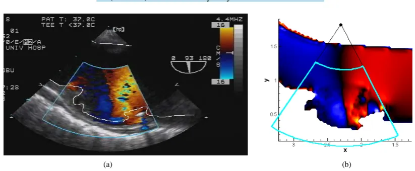
ment of an accurate diagnosis or treatment for circulatory diseases. A possible way to obtain such information is integration of numerical simulation and color Doppler ultrasonography in the framework of the flow field ob-server. Funamoto et al. [16] proposed ultrasonic-measurement-integrated (UMI) simulation (Figure 15). They performed a numerical study on the fundamental characteristics of UMI simulation using a simple two-dimen- sional model problem for blood flow in an aorta with an aneurysm. The result of UMI simulation in the feed-back domain converged to the standard solution, even with the usual inevitable incorrect upstream boundary conditions. An example of UMI simulation with feedback from real color Doppler measurement also showed good agreement with measurement (Figure 16).

Ultrasonic-measurement-integrated (UMI) simulation to reproduce three-dimensional steady and unsteady blood flows in an aneurysmal aorta with realistic boundary conditions was investigated [25] [30]. The transient characteristics of the UMI simulation were evaluated by the time constant or equivalently by the frequency re-sponse to the oscillating flow, and the steady characteristics were evaluated by the steady state error of the ve-locity vectors in an aneurysm. Veve-locity error vectors against the standard solution are shown inFigure 17[25]. In the initial state, the result is the same as that of the ordinary simulation with large error vectors. The error vectors decrease in and behind the feedback domain due to the effect of the feedback in the UMI simulation and converge to the steady state with small velocity errors.

Recently, Kato et al.[27] have developed an automated two-dimensional UMI (2D-UMI) blood flow analysis system for clinical diagnosis, and have investigated the feasibility of the system for hemodynamic analysis in a carotid artery. The system automatically generates a 2D computational domain based on ultrasound color Dopp-ler imaging and performs a 2D-UMI simulation of blood flow field to visualize hemodynamics in the domain. In the UMI simulation, compensation of errors was applied by adding feedback signals proportional to the differ-ences between Doppler velocities by measurement and computation, while automatically estimating the inflow velocity.

[image:13.595.202.429.402.515.2]

Magnetic resonance (MR)-measurement-integrated (MR-MI) simulation, in which the difference between the computed velocity field and the phase-contrast MRI measurement data is fed back to the numerical simulation,

Figure 15. Two-dimensional ultrasonic-measurement-integra- ted (2D-UMI) blood flow analysis system.

(a) (b)

[image:13.595.104.516.538.708.2]

has been also investigated [26]. The computational accuracy and the fundamental characteristics, such as steady and transient characteristics, of the MR-MI simulation were investigated by a numerical experiment for the three-dimensional steady and unsteady blood flow fields in a cerebral aneurysm developed at a bifurcation (Figure 18).

[image:14.595.160.465.152.293.2]

(a) (b)

Figure 17. Velocity error vectors of UMI simulation in (a) initial state and (b) con-vergent state [25].

(a) (b) (c)

Figure 18. Streamlines: (a) standard solution, (b) ordinary simulation and (c) MR-MI simulation [26].

4. Summary

In spite of the inherent difficulty, reproducing the exact structure of complex real flows is a critically important issue in many fields. In order to solve the problem, extensive studies have been carried out on methodology to integrate measurement and simulation. Measurement-integrated (MI) simulation, one of these methods, is a state observer in which a computational fluid dynamics (CFD) scheme is used as a mathematical model of the physi-cal system. A large dimensional nonlinear CFD model makes it possible to accurately reproduce real flows for properly designed feedback signal. This review article surveyed theoretical formulations and applications of MI simulation. Formulations of MI simulation were presented for governing equations of a flow field observer, li-nearized error dynamics, and stabilization of the numerical scheme. Applications of MI simulation were pre-sented ranging from fundamental turbulent flows in pipes and Karman vortices in a wind tunnel to clinical ap-plication to diagnosis of blood flows in a human body.

Acknowledgements

The author acknowledges former Transdisciplinary Fluid Integration Research Center, Advanced Fluid Informa-tion Research Center, and Institute of Fluid Science, Tohoku University for their support in establishing inte-grated research methodologies, including MI simulation.

References

[1] Imagawa, K. and Hayase, T. (2010) Numerical Experiment of Measurement-Integrated Simulation to Reproduce Tur-bulent Flows with Feedback Loop to Dynamically Compensate the Solution Using Real Flow Information. Computers

& Fluids, 39, 1439-1450. http://dx.doi.org/10.1016/j.compfluid.2010.04.012

[image:14.595.156.469.335.431.2]

[2] Thompson, J.M.T. and Stewart, H.B. (1986) Nonlinear Dynamics and Chaos. John Wiley and Sons, Hoboken.

[3] Benjamin, S.G., Devenyi, D., Weygandt, S.S., Brundage, K.J., Brown, J.M., Grell, G.A., Kim, D., Schwartz, B.E., Smirnova, T.G., Smith, T.L., et al. (2004) An Hourly Assimilation-Forecast Cycle: The RUC. Monthly Weather Re-view, 132, 495-518. http://dx.doi.org/10.1175/1520-0493(2004)132<0495:AHACTR>2.0.CO;2

[4] Zupanski, M. (1993) Regional 4-Dimensional Variational Data Assimilation in a Quasi-Operational Forecasting Envi-ronment. Monthly Weather Review, 121, 2396-2408.

http://dx.doi.org/10.1175/1520-0493(1993)121<2396:RFDVDA>2.0.CO;2

[5] Thepaut, J.N., Hoffman, R.N. and Courtier, P. (1993) Interactions of Dynamics and Observations in a 4-Dimensional Variational Assimilation. Monthly Weather Review, 121, 3393-3414.

http://dx.doi.org/10.1175/1520-0493(1993)121<3393:IODAOI>2.0.CO;2

[6] Bergamaschi, P., Frankenberg, C., Meirink, J.F., Krol, M., Villani, M.G., Houweling, S., Dentener, F., Dlugokencky, E.J., Miller, J.B., Gatti, L.V., et al. (2009) Inverse Modeling of Global and Regional CH4 Emissions Using SCIAMACHY Satellite Retrievals. Journal of Geophysical Research-Atmospheres, 114, D222301.

http://dx.doi.org/10.1029/2009JD012287

[7] Humphrey, J.A.C., Devarakonda, R. and Queipo, N. (1993) Interactive Computational-Experimental Methodologies (ICEME) for Thermofluids Research: Application to the Optimized Packaging of Heated Electronic Components. In: Yang, K.T. and Nakayama, W., Eds., Computers and Computing in Heat Transfer Science and Engineering, CRC Press and Begell House, New York, 293-317.

[8] Zeldin, B.A. and Meade, A.J. (1997) Integrating Experimental Data and Mathematical Models in Simulation of Physi-cal Systems. AIAA Journal, 35, 1787-1790. http://dx.doi.org/10.2514/2.31

[9] Ido, T., Murai, Y. and Yamamoto, F. (2002) Postprocessing Algorithm for Particle-Tracking Velocimetry Based on El-lipsoidal Equations. Experiments in Fluids, 32, 326-336. http://dx.doi.org/10.1007/s003480100361

[10] Uchiyama, M. and Hakomori, K. (1983) Measurement of Instantaneous Flow-Rate through Estimation of Velocity Profiles. IEEE Transactions on Automatic Control, 28, 380-388. http://dx.doi.org/10.1109/TAC.1983.1103235

[11] Sorenson, H.W., Ed. (1985) Kalman Filtering: Theory and Application. IEEE Press, New York.

[12] Högberg, M., Bewley, T.R. and Henningson, D.S. (2003) Linear Feedback Control and Estimation of Transition in Plane Channel Flow. Journal of Fluid Mechanics, 481, 149-175. http://dx.doi.org/10.1017/S0022112003003823

[13] Hayase, T. and Hayashi, S. (1997) State Estimator of Flow as an Integrated Computational Method with the Feedback of Online Experimental Measurement. Journal of Fluids Engineering-Transactions of the ASME, 119, 814-822. http://dx.doi.org/10.1115/1.2819503

[14] Nisugi, K., Hayase, T. and Shirai, A. (2004) Fundamental Study of Hybrid Wind Tunnel Integrating Numerical Simu-lation and Experiment in Analysis of Flow Field. JSME International Journal Series B Fluids and Thermal Engineer-ing, 47, 593-604. http://dx.doi.org/10.1299/jsmeb.47.593

[15] Hayase, T., Nisugi, K. and Shirai, A. (2005) Numerical Realization for Analysis of Real Flows by Integrating Compu-tation and Measurement. International Journal for Numerical Methods in Fluids, 47, 543-559.

http://dx.doi.org/10.1002/fld.829

[16] Funamoto, K., Hayase, T., Shirai, A., Saijo, Y. and Yambe, T. (2005) Fundamental Study of Ultrasonic-Measurement- Integrated Simulation of Real Blood Flow in the Aorta. Annals of Biomedical Engineering, 33, 415-428.

http://dx.doi.org/10.1007/s10439-005-2495-2

[17] Skelton, R. (1988) Dynamic Systems Control. John Wiley & Sons, New York.

[18] Misawa, E.A. and Hedrick, J.K. (1989) Nonlinear Observers—A State-of-the-Art Survey. Journal of Dynamic Systems,

Measurement, and Control-Transactions of the ASME, 111, 344-352. http://dx.doi.org/10.1115/1.3153059

[19] Curtain, R. and Zwart, H. (1995) An Introduction to Infinite-Dimensional Linear Systems Theory. Springer-Verlag, New York. http://dx.doi.org/10.1007/978-1-4612-4224-6

[20] Li, X. and Yong, J. (1995) Optimal Control Theory for Infinite Dimensional Systems. Birkhäuser, Boston. http://dx.doi.org/10.1007/978-1-4612-4260-4

[21] Imagawa, K. and Hayase, T. (2010) Eigenvalue Analysis of Linearized Error Dynamics of Measurement Integrated Flow Simulation. Computers & Fluids, 39, 1796-1803. http://dx.doi.org/10.1016/j.compfluid.2010.06.008

[22] Hayase, T., Imagawa, K., Funamoto, K. and Shirai, A. (2010) Stabilization of Measurement-Integrated Simulation by Elucidation of Destabilizing Mechanism. Journal of Fluid Science and Technology, 5, 632-647.

http://dx.doi.org/10.1299/jfst.5.632

[23] Nakao, M., Kawashima, K. and Kagawa, T. (2009) Application of MI Simulation Using a Turbulent Model for Un-steady Orifice Flow. Journal of Fluids Engineering-Transactions of the ASME, 131, 111401.

[24] Yamagata, T., Hayase, T. and Higuchi, H. (2008) Effect of Feedback Data Rate in PIV Measurement-Integrated Simu-lation. Journal of Fluid Science and Technology, Special Issue on Advanced Fluid Information, 3, 477-487.

[25] Funamoto, K., Hayase, T., Saijo, Y. and Yambe, T. (2009) Numerical Experiment of Transient and Steady Characteris-tics of Ultrasonic-Measurement-Integrated Simulation in Three-Dimensional Blood Flow Analysis. Annals of

Biomed-ical Engineering, 37, 34-49. http://dx.doi.org/10.1007/s10439-008-9600-2

[26] Funamoto, K., Suzuki, Y., Hayase, T., Kosugi, T. and Isoda, H. (2009) Numerical Validation of MR-Measurement- Integrated Simulation of Blood Flow in a Cerebral Aneurysm. Annals of Biomedical Engineering, 37, 1105-1116. http://dx.doi.org/10.1007/s10439-009-9689-y

[27] Kato, T., Funamoto, K., Hayase, T., Sone, S., Kadowaki, H., Shimazaki, T., Jibiki, T., Miyama, K. and Liu, L. (2014) Development and Feasibility Study of a Two-Dimensional Ultrasonic-Measurement-Integrated Blood Flow Analysis System for Hemodynamics in Carotid Arteries. Medical & Biological Engineering & Computing, 52, 933-943. http://dx.doi.org/10.1007/s11517-014-1193-3

[28] Patankar, S.V. (1980) Numerical Heat Transfer and Fluid Flow. Hemisphere Pub. Corp., McGraw-Hill, Washington DC, New York.

[29] Watkins, D.S. (1991) Fundamentals of Matrix Computations. Wiley, New York.

[30] Funamoto, K., Hayase, T., Saijo, Y. and Yambe, T. (2008) Numerical Experiment for Ultrasonic-Measurement-Integrated Simulation of Three-Dimensional Unsteady Blood Flow. Annals of Biomedical Engineering, 36, 1383-1397.