Interaction between vertical and horizontal tax competition: evidence and some theory

Munich Personal RePEc Archive

Interaction between vertical and

horizontal tax competition: evidence and

some theory.

Rizzo, Leonzio

Università degli studi di Ferrara

2007

Online at

https://mpra.ub.uni-muenchen.de/8632/

Interaction between vertical and horizontal tax

competition: evidence and some theory

Leonzio Rizzo

Abstract

The aim of this paper is to determine to what extent and how federal taxes affect local tax decisions. Testing the impact of an increase in the federal tax on horizontal tax competition with Canada-US data for 1984— 1994, wefind evidence that an increase in federal tax affects horizontal tax competition. The novelty of our approach is that it indirectly tests the effect of an increase in federal tax on provincial tax, by testing whether provincial reaction to an increase in neighboring tax changes according to the federal tax level. The test allows for control of yearly macroeconomic shocks by inserting dummies for each year. These are not used in the empirical literature on vertical tax competition because they would cause perfect collinearity with the federal tax.

Keywords: horizontal externality, vertical externality, tax competi-tion, tax rate.

JEL classification: H21.

1

Introduction

Federal tax isfixed in the cross section and does not normally vary by province or state. The literature regresses local tax rate on the federal tax rate as Besley and Rosen (1998) do,finding a positive coefficient. This method prevents checking for year effects, because the federal tax rate in a panel data set does not have a state dimension, and insertion of year effects results in an insignificant coefficient for the federal tax rate, which is a linear combination of year effects. The typical problem in these studies is that the federal tax-coefficient can be significant because it picks up yearly macroeconomic shocks. Esteller-Moré and Solé-Ollé (2001) analyzed the vertical externality for the US using a state average federal income tax rate instead of the marginal federal tax rate. The tax rate calculated in this way

∗_{University of Ferrara, Department of Economics, Via Voltapaletto 11, 44100, Ferrara.}

1_{I wish to thank Tim Besley, Umberto Galmarini, Jim Hines, Valentino Larcinese and Cecilia}

varies by state, so that the method is able to control for year effects. They also find a positive coefficient. Andersson et al. (2004) test the presence of vertical externality on income tax rates using data on the Swedish local and regional public sector for the period 1981-1990. In this case they are able to control for yearfixed effects because their high jurisdiction tax level varies by counties, which are 24: they find a negative coefficient.

Interestingly, some recent studies put together horizontal and vertical fiscal externalities with contrasting results. Goodspeed (2000) used a data set with 13 OECD provinces for the period 1975—1984. A poverty index was used as a mea-sure of intra-province mobility: the poorer the less mobile people are, the smaller is the horizontal externality. The author used local income tax as a dependent variable and found a negative sign for the federal tax rate and for the mobility index. Boadway and Hayashi (2001), using Canadian annual data for 1963—1996, tested horizontal and vertical tax competition by considering corporate taxes on businesses. They found a negative sign for the vertical externality and positive sign for the horizontal externality. Each estimate was for a single province or an average province. This result is confirmed by Karkalakos, Kotsogiannis (2007), who extend the previous work exploring fiscal interactions for all ten fiscal au-tonomous provincial governments. Revelli (2003) studied the non-metropolitan two-tier system of local government in England–comprising 34 counties and 238 districts–using per capita current expenditure for thefinancial year 2000/2001, disaggregated into various functions of interest. He found that horizontal exter-nality disappears when a vertical exterexter-nality coefficient is introduced, arguing that the only relevant externality is the last one. Interestingly, Devereux et al. (2007) found the opposite for the US using panel data for 1977—1997: vertical externality for cigarette and gasoline taxes was not significant if there was also a test for horizontal externality, which was significant. None of these studies, even if controlling for neighboring taxes, have checked for year effects. Finally Brulhart and Jametti (2006) use a local-regional panel data and build an income tax rate index for Switzerland for the years 1985, 1991, 1995 and 1998. They find a positive link between the tax chosen by the canton and that chosen by the municipality, and that vertical tax externality prevails over horizontal tax externality. They obtain this latter result by using an indirect estimate of the sum of these two esternalities through a "smalleness" index of the municipality. They can control for year effects because, as in Andersson et al. (2004), the high jurisdiction tax level varies by canton, of which there are 23 in their panel.

the vertical externality affects the horizontal externality (measured through a poverty index; Goodspeed, 2000) in an income tax environment by offsetting it. In his study, differently from the present one, there was no check for year effects. Moreover, the present study uses tax rates rather than the ratio of tax revenue to GNP; it also does not estimate the horizontal externality, but the tax competition coefficient and interacts the independent tax variable (the mean of the taxes of the neighbors) with the federal tax variable. It finds that the federal tax rate affects the neighboring average tax rate in explaining the variance of a province’s own tax rate.

The remainder of the paper is organized as follows: the second section re-ports an empirical test. Section 3 outlines a theoretical model and explains the empirical results. Section 4 concludes.

2

The empirical test

We use a Canada2_{—US data set for 1984—1994 to estimate if there is any significant}

strategic link between federal and provincial taxation when tax is levied on the same tax base. In the literature this has been carried out by regressing the local tax rate on the federal tax rate (Besley and Rosen, 1998). It should be noted that the federal tax coefficient can be significant because it picks up a year, or trend effect. Onfirst glance at our data, it seems that both situations are particularly true. Fig. 1 shows trends, normalized by province, for Canadian provincial, federal and mean neighboring taxes on cigarettes, expressed in 1989 US$. The three variables are well correlated for every province and trend up to 1993. From 91 to 93 there was a strong federal no-smoking policy and federal taxes increased, followed by provincial taxes as well. In 1994, federal tax was drastically cut to counteract smuggling from the US; almost all provinces adopted the cut. We conclude that the federal tax effect cannot be estimated by omitting year effects, which also allow for control for the trend effect.3

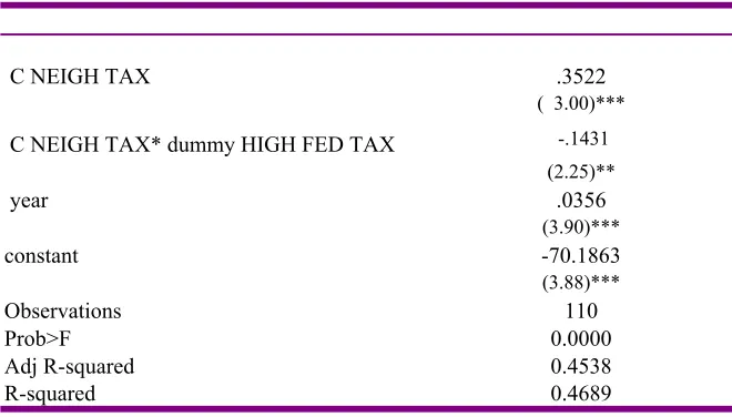
We split the sample into two subsamples. One subsample is relative to the years when the federal tax on cigarettes, expressed in 1989 US$, is low (this the period 1984—1990 and 1994 when the federal tax was less than 0.462 per pack of 20 cigarettes) and the other subsample relates to the years when the federal tax on cigarettes is high (it is the period 1991—1993: the federal tax was larger than 0.894 per pack of 20 cigarettes). To understand whether there are some regularities in the tax-rates relations of the subsamples considered, we regress each province’s own tax on the average of the neighboring Canadian taxes and interact this coefficient with a dummy equal to 1 for the high federal tax subsample and control for the time trend. Table 2 shows that the tax competition coefficient is

2_{We excluded the three territories of Nunavut, Northwest Territories and Yukon because}

lower when the federal tax is high (0.3522-0.1431) than when it is low (0.3522): the interaction coefficient is negative (-0.1431).

This preliminary check suggests that the provincial tax reaction to a change in the mean neighboring provincial tax changes according to the federal tax level, supporting the idea that the federal tax matters in provincial tax decisions. If the federal authority intervenes by introducing a central tax, it affects the local welfare and the choice of the provincial tax, and thus the tax-rate response to an increase in tax rate in a neighboring province. The next sections investigate this issue in more detail.

2.1

Estimation Strategy

To isolate the independent impact of the neighboring tax rates on Canadian provincial tax, the other variables that might affect the provincial tax rates must be taken into account. Therefore, we control for the US neighboring tax rates. Moreover the provincial tax rate on goods depends on several other types of vari-ables. Provincial taxation may be influenced by the economic and demographic environment. We controlled for this by using socioeconomic variables (see data appendix). For all of these variables we computed the corresponding mean vari-able for the neighboring Canadian provinces and neighboring US states for each Canadian province. The political party of the provincial government may also affect the tax-rate level: we divided the Canadian party system into three main groups: the conservative-progressive group, which is right wing; the liberal group, which is center; and the left wing group, comprising the Democratic-Progressives, the Quebec party and the Social Credit party. We then build two dummies ac-counting for the premier of the province being liberal or conservative-progressive. Finally, we have dichotomous variables to control for province and year effects. We check the effect of federal tax on the tax competition coefficient by estimating the following equation on the entire data set:

tst =αs+βt+γ1hst+γ2vthst+γ3mst+θxst+ st (1)

where: tstis the tax rate for provinces and yeart;αs is the province fixed effect;

hstis the tax-rate average for the provinces neighboring province sin yeart;vt is

the federal tax rate in year t; mst is the tax-rate average of the US states

neigh-boring province s in year t; xst is a vector of the province-specific time-varying

variables P OPst, CHILDst, AGEDst, GRANTst, UN EMPst, INC, IN C2; the

corresponding Canadian and US neighboring variables forINCst andINCst2

com-puted respectively as hst and mst; the dummies for the premier of the province

being liberal or conservative-progressive and st is the error term.

Note that γ1+γ2vt is the slope of the tax-rate reaction function for a given

mean of the federal tax. After the results of the preliminary check reported in the previous section, we may want to test γ2 <0: an increase in the federal tax

2.1.1 Instrumentation

The mean Canadian neighboring tax rate and its interactions are endogenous, because they can also be influenced by the Canadian provinces. The mean neigh-boring US tax rate, mst may clearly be endogenous: the US rate mean may also

be influenced by the Canadian provinces.

If this is a structural model, a simple OLS estimate of (1) would suffer from endogeneity bias: the error term st would be correlated with the error terms of

the other simultaneous equations of the system. The endogeneity bias arises from the fact that we are dealing with simultaneous equations. We use the two-stage least squares method: first we estimate the reduced forms of the endogenous variables and then substitute their fitted values into (1). The residuals of this last equation are corrected using the actual values of the endogenous variables.4

We instrumented the mean Canadian neighboring tax ratehst with the

neigh-boring Canadian variables forAGEDst,vthstfirstly withAGEDst andUNEMPst,

interacted with vt and secondly with AGEDst and UNEMPst, interacted with

F ED UNEMPt.5 Finally, we instrumented the mean US neighboring tax rate

with the US neighboring variables for P OPst

In a reduced-form equation, the tax rate on cigarettes is reasonably linked to the size of the population: this variable influences the available tax base and the cost of public goods. Moreover, the age structure influences taxation according to the relative preference for social policies. It is reasonable to think that these neighboring variables do not affect the provincial tax rate on cigarettes. The economic cycle is also important in determining the tax rate level, and this is captured by UNEMPst.

Wefinally have 4 instruments, and therefore Eq. (1), which has three endoge-nous variables, is identified.

Moreover, in the second-stage equation we also control for demographic vari-ablesP OPst,CHILDst,AGEDst and variables controlling for the economic cycle

likeGRANTst, UNEMPst, INCst and INCst2.

Spatial error dependence may arise when the error includes some omitted vari-ables not captured in the covariates, which are themselves spatially dependent. If the spatial dependence is ignored the estimation may be biased (Brueckner, 2001; Brueckner and Saavedra, 2001). We deal with this problem by controlling

4_{The two-stage least squares strategy would deliver residuals using thefitted values of the}

endogenous variables. Since we are estimating a structural model, we are interested in the residuals using the actual values of the endogenous variables.

We execute the procedure using the ivreg2 command of STATA, which already gives the corrected residuals with the actual values of the endogenous variables.

5_{In thefirst case we estimate a Stackelberg model where the federal government movesfirst}

for a variable proxying the neighboring economic environment: the neighboring Canadian variables for INCst and its square, and symmetric variables for the

neighboring US states. If those variables are omitted, they may generate a spu-rious correlation between a province’s own tax and the neighboring tax or other exogenous covariates.

After performing the two-stage least squares regressions, we test the validity of the instruments using the Hansen J-test,6 _{the minimized value of the GMM}

criterion function. The joint null hypothesis is that the excluded instruments are valid instruments, i.e., uncorrelated with the error term, and that they are correctly excluded from the estimated equation. Under the null, the test statistic is distributed as χ2

in the number of overidentifying restrictions.

2.2

Results

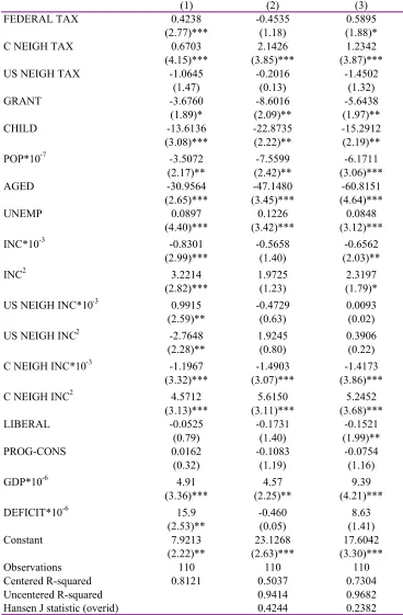
Table 3 first reports a simple OLS regression (column 1) that tests for vertical and horizontal externalities: the coefficients are both positive and significant at the 1% level. In this regression we control for province effects and take account of trends or macroeconomic shocks using federal GDP and deficit. When we instru-ment the Canadian and US average neighboring taxes (column 2), the federal tax is not significant and the overidentification test is not satisfactory (P = 0.42). Column 3 shows a specification whereby the federal tax is instrumented with the federal unemployment. The federal tax coefficient increases, becoming significant at the 10% level and the overidentification test is worse (P = 0.22). This means that the instruments are not good, or that the specification is not correct because some variable correlated with the instruments is missing. We opt for the second argument and estimate a model with year effects, dropping the federal tax coef-ficient. We adopt a specification whereby the federal tax is interacted with the mean of the neighboring taxes. Specifically (Table 4) we estimate the horizontal tax-competition coefficient: γ1+γ2vt. This is the slope of the tax-rate reaction

function, and the interesting coefficient is γ2.

In Table 4γ2 =−3.51is negative and significant at the 1% level, meaning that

an increase in federal tax decreases the tax reaction to an increase in the mean of the neighboring taxes. Finally, the overidentification test greatly improves (P = 0.76), supporting the idea that the interaction term and the year effects were really missing variables. We also checked a model assuming the federal

6_{The Hansen-Sargan test is a test of overidentifying restrictions. For the efficient GMM}

estimator, the test statistic is Hansen’sJ-statistic, the minimized value of the GMM criterion function. For the 2SLS estimator, the test statistic is Sargan’s statistic, typically calculated as N ×R2 _{from a regression of the IV residuals on the full set of instruments. TheJ-statistic}

tax as endogenous, instrumenting the federal tax interaction with the federal unemployment, and the result did not change (column 2 of table 4)

3

Making sense of the results

Consider a federation with two provinces and a federal government maximizing their welfare functions. One mobile good is produced using one input with a constant return to scale technology. The good is taxed according to the desti-nation principle. Using the same tecnology a good not mobile is also produced. This good is not taxed. The production cost of the two goods is normalized to 1. When the destination principle (people pay tax where they consume the good) holds, cross-border shopping for the taxed good may occur.

We model the interaction between the federal government and the province as a Stackelberg game (Boadway et al., 1998; Keen and Kotsogiannis, 2002). Let i = 1,2 index the two provinces. In the first stage, the central government chooses the federal taxT by maximizing its welfare, and in the second stage each province chooses its tax rateti, by maximizing its own welfare, given the federal

tax choice. Each citizen in province i hasmi+ 1 units of endowments; she uses

one unit to pay the net of tax price of the taxed good, with inelastic demand equal to 1. With the remaining units she pays taxes on the mobile good and consumes the other good. Each citizen can move to buy the mobile good in the province where it is cheaper, bearing a transport cost δ per unit of distance d. We solve the model by backward induction.

3.1

The consumer decision

Let ti be the specific unit tax on the mobile good, levied by provincei. Assume

thatt1 > t2. The consumer in province 1 decides where to buy the good according

to her net surplus. If the customer buys in province 1, she pays t1 plus the

production cost. If the customer crosses the border and buys in province 2, she pays d+t2 plus the production cost. Therefore consumer in province 1 will shop

from province 2 until:

d1δ+t2 =t,

then:

d1 =

t1−t2

δ , (2)

where d1 is the distance from the border of the consumer in province 1, who is

is also the number of residents in province 1, buying goods from province 2, for a given t1−t2.

If t1 ≤t2, analogously we obtain:

d2 =

t2−t1

δ , (3)

where d2 is the distance from the border of the consumer in province 2, who

is indifferent between shopping in province 2 or cross the border and shop in province 1. d2 is also the number of residents in 2, buying from province 1, for a

given t2−t1.

Finally, if t1 > t2:

B1 = 1−d1, (4)

and if t1 ≤t2:

B1 = 1 +d2, (5)

where B1 is the tax base faced by province 1, whose population is normalized to

1. We can simplify the notation by defining:

n(t1, t2) =

½

−d1 if t1 > t2

d2 if t1 ≤t2.

(6)

It follows that:

B1 = 1 +n(t1, t2), (7)

and:

B2 = 1−n(t1, t2), (8)

where n is the incoming or outgoing mobile tax-base quota depending on which tax regime we are dealing with.

3.2

The province problem

At the second stage provincei maximizes the following function:

Wi = ln µ

1₋ ti−tj δ

¶

ti+ ln (mi−T −ti) +γ(1) lnu, (9)

with i 6= j. The first term is the utility from revenue collected by the province taxing the good; the second term is the utility for the representative citizen, from consumption of the good not taxed, after paying federal and provincial tax and buying the taxed good in her province; the third term is the utility from consumption of the taxed good, x with γ(x) = 1 if x≥1 andγ(x) = 0 if x <1

andfinally u >1.7 _{These assumptions imply that the demand for the good x is}

inelastic and equal to one. (See appendix only for the referee)

Provincial taxation of the mobile good is distorted by the mobility incentive

and the presence of a higher layer of government. In particular, if the province tax rate on the good x is equal to ti, tax revenue for province i is equal to

ti ³

1₋ ti−tj

δ ´

, but the burden for taxpayers (in terms of forgone consumption of the other good) is equal to(mi−T −ti), because taxpayers bear also the federal

tax T. Note that (9) implies that the province cares about revenue and the indirect utility of a representative citizen buying the taxed good in her province. In particular the second term of (9) implies that the larger ti and/or T, the

smaller the utility from the endowment quota available to buy the other good.

At the first stage the federal government solves the following problem:

Max

T ln 2T +

2

X

i=1

ln

µ

1₋ t

∗

i −t∗j

δ

¶

t∗_i +

2

X

i=1

ln (mi−T −t∗i)

Where t∗

i and t∗j are second stage tax rates equilibrium. Notice that a subgame

perfect equilibrium must necessarily deliver:

ti−tj

δ <1 (10)

and

mi−T −ti >0. (11)

3.3

The reaction function

Let us explore the second stagefirst order conditions. Provinceichoosesti, which

maximizes (9), obtaining the following first order condition:

dWi

dti

= δ−2ti+tj δti−t2i +titj −

1 mi−T −ti

= 0, (12)

it follows:

(δ−2ti +tj) (mi−T −ti)−(δ−ti+tj)ti = 0, (13)

Implicitly differentiating (13) with respect to ti and tj and defining A =

T + 2ti−mi:

dti

dtj

= A

2 (A+ti−tj −δ)

>0. (14)

Proof: (10) and (11) imply that if (13) holds then:

Moreover, sinceδ₋2ti+tj < δ−ti+tj, then, when (13) holdsmi−T −ti > ti,

which is:

A = 2ti+T −mi <0. (16)

Finally using (15) and (11):

A+ti−tj −δ= 2ti−tj −δ−(mi−T −ti)<0. (17)

Use of (16) and (17) implies the sign of (14).

Implicit differentiation with respect to ti andT of (13) gives:

dti

dT =−

δ₋2ti+tj

2 (A+ti−tj−δ)

. (18)

Since we know from above thatA+ti−tj−δ <0, and from (15) we know that

the numerator of (18) is positive, then dti

dT >0.

How does the existence of a federal tax on the same tax base affect the reaction function of one provice with respect to the other province tax rate? To answer this question we must compute the following derivative of (14) with respect toT, at the second stage tax-rates equilibrium:

dti

dtjdT

=

(ti−tj −δ)¡1 + 2dt_dTi¢−A ³

dti

dT − dtj

dT ´

2 (A+ti −tj−δ)

2 <0.

This holds in the symmetric case (m1 = m2) and also in the asymmetric case

(m1 6=m2) if the distance between m1 andm2 is not too big.

4

Conclusions

We have tested the impact of an increase in federal tax on tax competition, providing evidence that an increase in federal tax affects tax competition, since provinces behave differently after an increase in federal tax. Federal tax matters, because it affects the welfare of the province: that is, it decreases the sensitivity of the province tax to a change in tax of the neighboring provinces.

The novelty of this approach is that one can indirectly test the effect of an increase in federal tax on the provincial tax by controlling for yearly macroeco-nomic shocks, which are not used in the standard empirical literature because they would be perfectly collinear with the federal tax. We accordingly test the coefficient of the variable for the interaction between federal tax and the mean of the neighboring taxes. The paper developed a test using a data set for Canada and US running from 1984 to 1994 for specific cigarette taxes.

each state fixes its tax rate, being aware of the neighboring rates, where popu-lation density near the border and the length of the border are greater. From a theoretical point of view, it would be interesting to explore the political economy reasons that could determine the ambiguous sign of the vertical externality re-ported previously in the literature: friendly provinces could decide to sustain the federal authority’s decision to increase the federal tax by decreasing their own, while other, non-friendly provinces could do the opposite.

References

[1] Andersson, L., Aronsson T., Wikstrom M. (2004), Testing for Vertical Ex-ternalities, Internaltional Tax and Public Finance, 11, 243-263.

[2] Besley, T. and H. S. Rosen (1998), Vertical externalities in tax setting: evi-dence from gasoline and cigarettes, Journal of Public Economics 70, 383-398. [3] Boadway, R. and M. Hayashi (2002), An Empirical Analysis of Intergov-ernmental Tax Interaction: the Case of Business Income Taxes in Canada, Canadian Journal of Economics, 34, 481-503.

[4] Boadway, R., Marchand M., Vigneault M. (1998), The Consequences of Overlapping Tax Bases for Redistribution and Public Spending in a Fed-eration, Journal of Public Economics, 68, 453-478.

[5] Brueckner, J. K. (2003) Strategic Interaction Among Governments: An Overview of Empirical Studies, International Regional Science Review, 26, 175-188.

[6] Brueckner, J. and Saavedra, L. A. (2001) Do Local Governments Engage in Strategic Property-Tax Competition?, National Tax Journal, 54, 203-229. [7] Brulhart, M. and Jametti, M. (2006), Vertical versus Horizontal Tax

Exter-nalities: an Empirical Test, Journal of Public Economics, 90, 2027-2062. [8] Devereux, M.P., Lockwood B., Redoano M. (2007). Horizontal and vertical

indirect tax competition: Theory and some evidence from the USA, Journal of Public Economics, 91, 451-479.

[9] Esteller-Moré A. and A. Solé-Ollé (2001), Vertical Income Tax Externalities and Fiscal Interdependence: Evidence from the US, Regional Science and Urban Economics, 31, 247-272.

[11] Goodspeed, T J. (2000), Tax Structure in a Federation, Journal of Public Economics, 75, 493-506.

[12] Goodspeed, T J. (2002), Tax competition and tax structure in open fed-eral economies: Evidence from OECD provinces with implications for the European Union, European Economic Review 46, 375-374.

[13] Karkalakos, S. and C. Kotsogiannis, (2007). A spatial analysis of provincial corporate income tax responses: evidence from Canada, Canadian Journal of Economics, 40, 782-811.

[14] Keen, M. (1998), Vertical Tax Externality in the Theory of Fiscal Federalism, IMF StaffPapers 45, 454-485.

[15] Keen, M. and C. Kotsogiannis (2002), Does federalism lead to excessively high taxes?, American Economic Review, 92, 363-369.

[16] Peitz, M. (1995), Utility maximization in models of discrete choice, Economic Letters, 49, 91-94.

[17] Revelli, F.(2003), Reaction or Interaction? Spatial Process Identification in Multi-tiered Government Structures, Journal of Urban Economics, 53, 29-53.

5

Data Appendix

tst Canadian cigarette tax rate, for provincesin year t,divided by the Canadian

CPI and the Canada-US PPP index; these rates are provided by the Finance departments of the ten considered provinces and are expressed in Canadian dollars per pack of 20 cigarettes.

5.1

Endogenous variables

vt is the federal Canadian cigarette tax rate. This is from the National

Clearing-house on Tobacco and Health for Canada.

hst is the mean of the tax rates in yeart of the Canadian provinces bordering

on province s, divided by the Canadian CPI and the Canada-US PPP index.

mst mean of the tax rates of the US states bordering on province s in year

5.2

Demographic and economic variables

P OPst is the number of persons in province s in yeart. It is taken from www.

statcan.ca for Canada and www.census.gov for the US.

CHILD is the ratio of individuals aged 5—17 years to the total population of provinces in year t, taken from www.statcan.ca for Canada.

AGEDst is the ratio of individuals of over 65 years of age to the total

pop-ulation of province s in year t, taken from www.statcan.ca for Canada and www.census.gov for the US.

UNEMPst is the unemployment rate for province s in year t, taken from

www.statcan.ca for Canada and from www.stats.bls.gov for the US.

INCst is the per-capita income for province s in year t divided by the CPI

and PPP index. Income data were taken from www.statcan.ca.

GRANTstis the federal grant-in-aid over GDP for provincesin yeart. Federal

grant-in-aid data for Canada were taken from www.statcan.ca.

P ROG₋CONSst is dummy=1 if the premier of the province is Progressive

Conservatives, taken from http://www.swishweb.com/Politics/Canada.

LIBERALst dummy=1 if the premier of the province of Liberal Party, taken

from http://www.swishweb.com/Politics/Canada.

F ED GDP is the federal GDP for yeartdivided by the CPI and PPP index, taken from www.statcan.ca.

F ED UNEMP is the federal unemployment for year t, taken from www. statcan.ca.

F ED DEF ICIT is the federal deficit for yeart, taken from www.statcan.ca. The PPP (Parity Purchasing Power) index for Canada-US was downloaded from the OECD web site.

The US CPI was taken from the Statistical Abstracts of the United provinces (2000).

The Canadian CPI was taken from http://www.statcan.ca.

5.3

The neighboring variables

A neighboring Canadian variable for provincesin yeartis computed as the mean of the variable in all the Canadian provinces neighboring province s in year t.

The neighboring Canadian xvariable is defined as: C NEIGH x.

A neighboring United States variable for province s in year t is computed as the mean of the variable in all the US states neighboring province s in year t.

The neighboring United Statesx variable is defined as: US NEIGH x.

An example: suppose there are four neighboring provinces (defined as n = 2,3,4,5), then the neighboring Canadian xst variable for province 1 in year t

would be:

C NEIGH x1_t=

P s∈n

xst

6

Appendix only for the attention of the referee

The citizen buying the taxed good in her province solves the following problem:

max

x,y u(x, y) = lny+γ(x) lnu

s.t.:mi+ 1 = (1 +ti+T)x+y

(19)

Notice that by assumption if x_≥1then γ(x) = 1,implying that the solution of the optimization problem is x = 1; substituting the budget constraint with

x= 1 in the utility function:

v(1, mi−ti −T) = ln (mi −ti−T) + lnu. (20)

By assumption if x < 1 then γ(x) = 0, implying that the solution of the opti-mization problem is x= 0; substituting the budget constraint with x= 0 in the utility function:

v(0, mi+ 1) = ln (mi+ 1). (21)

The last step to solve (19) is comparing (20) with (21):

v(1, mi−ti−T)> v(0, mi+1) if and only if 1+ti+T <

(u−1) (mi + 1)

u . (22)

Condition (22) must be satisfied if a subgame perfect equilibrium , T, t1, t2,

with positive revenues holds. Hence the citizen buying the good in her province chooses:

y=mi−ti−T

and

Variable Observations Mean Std. Dev. Min Max

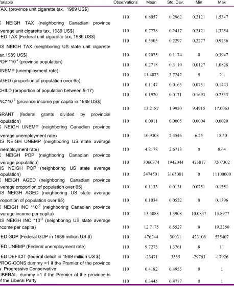
TAX (province unit cigarette tax, 1989 US$)

110 0.8057 0.2962 0.2121 1.5347

C NEIGH TAX (neighboring Canadian province

average unit cigarette tax, 1989 US$) 110 0.7778 0.2417 0.2121 1.3254

FED TAX (Federal unit cigarette tax, 1989 US$)

110 0.5505 0.2297 0.2277 0.9236

US NEIGH TAX (neighboring US state unit cigarette

tax,1989 US$) 110 0.2075 0.1174 0 0.3947

POP *10-7 (province population)

110 0.2718 0.3110 0.0127 1.0828

UNEMP (unemployment rate)

110 11.4873 3.7242 5 21

AGED (proportion of population over 65)

110 0.1147 0.0163 0.0751 0.1443

CHILD (proportion of population between 5-17)

110 0.1920 0.0171 0.1693 0.2533

INC*10-3 (province income per capita in 1989 US$)

110 13.2187 1.9920 9.4915 17.0063

GRANT (federal grants divided by provincial

population) 110 0.0011 0.0005 0.0004 0.0020

C NEIGH UNEMP (neighboring Canadian province

average unemployment rate) 110 10.9308 2.4546 6.25 15.50

US NEIGH UNEMP (neighboring US state average

unemployment rate) 110 4.8178 2.6718 0 8.64

C NEIGH POP (neighboring Canadian province

average population) 110 3060374 1942044 423817 7207302

US NEIGH POP (neighboring US state average

population) 110 2474501 3165001 0 11100000

C NEIGH AGED (neighboring Canadian province

average proportion of population over 65) 110 0.1133 0.0131 0.0751 0.1351

US NEIGH AGED (neighboring US state average

proportion of population over 65) 110 0.1034 0.0522 0 0.1396

C NEIGH INC *10-3 (neighboring Canadian province

average income per capita) 110 13.4088 1.3908 10.0837 15.8977

US NEIGH INC *10-3 (neighboring US state average

income per capita) 110 12.7175 6.5527 0 19.2380

FED GDP (Federal GDP in 1989 million US $) 110 476244 30031 423106 535407

FED UNEMP (Federal unemployment rate) 110 9.7273 1.3761 8 11

FED DEFICIT (federal deficit in 1989 million US $) 110 -23471 3535 -29763 -17926

PROG-CONS dummy =1 if the Premier of the province

is Progressive Conservative 110 0.4182 0.4955 0 1

LIBERAL dummy =1 if the Premier of the province is

of the Liberal Party 110 0.3445 0.4777 0 1

Table 1: Summary Statistics

C NEIGH TAX .3522 ( 3.00)***

C NEIGH TAX* dummy HIGH FED TAX -.1431

(2.25)**

year .0356

(3.90)***

constant -70.1863

(3.88)***

Observations 110

Prob>F 0.0000

Adj R-squared 0.4538

R-squared 0.4689

Notes:We splitted the sample into two subsamples, according to the federal tax.

A dummy for the high federal tax years (91-92-93) is interacted with the tax-competition coefficient. Numbers in parenthesis are t-statistics (with robust standard errors). Variables are defined in table 1 and described in detail in the data appendix.

* significant at 10%; ** significant at 5%; *** significant at 1%

Dependent variable: province cigarette tax (specific unit tax), 1984-1994.

Table 3: Federal tax (specific unit tax) on cigarettes.

(1) (2) (3)

FEDERAL TAX 0.4238 -0.4535 0.5895

(2.77)*** (1.18) (1.88)*

C NEIGH TAX 0.6703 2.1426 1.2342

(4.15)*** (3.85)*** (3.87)***

US NEIGH TAX -1.0645 -0.2016 -1.4502

(1.47) (0.13) (1.32)

GRANT -3.6760 -8.6016 -5.6438

(1.89)* (2.09)** (1.97)**

CHILD -13.6136 -22.8735 -15.2912

(3.08)*** (2.22)** (2.19)**

POP*10-7 -3.5072 -7.5599 -6.1711

(2.17)** (2.42)** (3.06)***

AGED -30.9564 -47.1480 -60.8151

(2.65)*** (3.45)*** (4.64)***

UNEMP 0.0897 0.1226 0.0848

(4.40)*** (3.42)*** (3.12)***

INC*10-3 -0.8301 -0.5658 -0.6562

(2.99)*** (1.40) (2.03)**

INC2 3.2214 1.9725 2.3197

(2.82)*** (1.23) (1.79)*

US NEIGH INC*10-3 0.9915 -0.4729 0.0093

(2.59)** (0.63) (0.02)

US NEIGH INC2 -2.7648 1.9245 0.3906

(2.28)** (0.80) (0.22)

C NEIGH INC*10-3 -1.1967 -1.4903 -1.4173

(3.32)*** (3.07)*** (3.86)***

C NEIGH INC2 4.5712 5.6150 5.2452

(3.13)*** (3.11)*** (3.68)***

LIBERAL -0.0525 -0.1731 -0.1521

(0.79) (1.40) (1.99)**

PROG-CONS 0.0162 -0.1083 -0.0754

(0.32) (1.19) (1.16)

GDP*10-6 4.91 4.57 9.39

(3.36)*** (2.25)** (4.21)***

DEFICIT*10-6 15.9 -0.460 8.63

(2.53)** (0.05) (1.41)

Constant 7.9213 23.1268 17.6042

(2.22)** (2.63)*** (3.30)***

Observations 110 110 110

Centered R-squared 0.8121 0.5037 0.7304

Uncentered R-squared 0.9414 0.9682

Hansen J statistic (overid) 0.4244 0.2382

* significant at 10%; ** significant at 5%; *** significant at 1%

Dependent variable: province cigarette tax (specific unit tax), 1984-1994.

(1) (2)

C NEIGH TAX 2.5991 4.0504

(2.72)*** (1.94)*

C NEIGH TAX * FED TAX -3.5144 -5.8663

(2.80)*** (1.97)**

US NEIGH TAX -1.0637 -3.5116

(0.79) (1.34)

GRANT -7.3861 -6.9936

(3.37)*** (2.48)**

CHILD -9.8944 -12.3094

(1.67)* (1.20)

POP*10-7 -4.9865 -4.8764

(3.61)*** (2.61)***

AGED -39.7100 -37.0020

(3.30)*** (2.08)**

UNEMP 0.0872 0.0994

(3.76)*** (2.40)**

INC*10-3 -0.5921 -0.4365

(2.03)** (1.32)

INC2 2.1018 1.4562

(1.76)* (1.10)

US NEIGH INC*10-3 0.4739 0.1198

(0.81) (0.17)

US NEIGH INC2 -1.0756 0.2519

(0.56) (0.11)

C NEIGH INC*10-3 -1.1684 -1.2181

(3.48)*** (2.47)**

C NEIGH INC2 4.1917 4.4510

(3.07)*** (2.15)**

LIBERAL -0.0603 -0.0746

(0.99) (0.79)

PROG-CONS -0.0002 0.0579

(0.00) (0.62)

Constant 12.8172 14.5301

(3.61)*** (2.61)***

Observations 110 110

Centered R-squared 0.8057 0.6600

Uncentered R-squared 0.9771 0.9598

Hansen J statistic (overid) 0.7617 0.7179

* significant at 10%; ** significant at 5%; *** significant at 1%

Table 4: The impact of federal tax on horizontal tax competition.

Dependent variable: province cigarette tax (specific unit tax), 1984-1994.

0

.5

1

0

.5

1

0

.5

1

1985 1990 1995 1985 1990 1995

1985 1990 1995 1985 1990 1995

ALB BC MAN NB

NFDL NS ONT PEI

QUE SASK

FED_TAX TAX

C_NEIGH_TAX

Ta

x

r

a

te

s

year

Graphs by stcode