Algorithm Analysis of Numerical Solutions to the Heat
Equation
Edmund Agyeman
Department of Mathematics, Kwame Nkrumah University of Science and
Technology, Kumasi-Ghana.
Derick Folson
Department of Mathematics, Kwame Nkrumah University of Science and
Technology, Kumasi-Ghana.
ABSTRACT
The numerical algorithms employed in the solution of Parabolic Partial Differential Equations are the subject of this paper. In particular, the Crank-Nicolson scheme, which is generally accepted as an improvement of the Schmidt scheme, is subjected not only to stability analysis, but also absolute relative error analysis to guide Mathematicians and Engineers alike to know the true performance of these numerical solution methods. The Heat Equation with Dirichlet conditions conducting heat is analysed by employing the analytical method of solution where the method of Separation of Variables is used. The same equation is then solved with the Schmidt scheme as well as the Crank-Nicolson scheme and the results compared to the analytical solution.
It is shown that provided stability conditions for both numerical schemes are not compromised, the Schmidt scheme is better than the Crank-Nicolson scheme at the particular point 80% from the conducting end of the rod. With the rod discretized into six points, both ends of the rod produce the same results for both numerical schemes. With the remaining four points, it is shown that three points produced values which showed that the Crank-Nicolson scheme is better than the Schmidt scheme at those three points, but not the fourth.
General Terms
Numerical Solution, Finite Difference, Relative Absolute Error, Parabolic PDEs, Separation of Variables, Dirichlet condition, Crank-Nicolson scheme, Schmidt scheme, Stability
Keywords
Numerical Analysis, Algorithm, Heat Equation
1. INTRODUCTION
Numerical mathematics has come to the aid of mathematicians for centuries and has made the solution of otherwise unsolvable mathematical problems quite easy. This has been felt in almost all branches of Science especially, mathematics, engineering and medicine.
When numerical mathematics reached its peak in the mid 20th century, among those who made their names were the German scholar Erhard Schmidt (forming the Schmidt method), English Mathematical mathematicians John Crank and Phyllis Nicolson (together forming the Crank-Nicolson method). These outstanding mathematicians of old proposed algorithms for solving partial differential equations numerically.
Even though these algorithms are used widely today in almost all fields of Science, time has come to put these algorithms under the lens for informed decision to be made on them. Although quite some steps have been taken by various mathematicians to analyse these algorithms, all effort unfortunately focus only on their stability analysis.
2. OBJECTIVES
This paper among other things seeks to:
Apply analytical and numerical methods to solve a parabolic partial differential equation.
Compare the numerical solutions to the analytical solution and draw informed conclusions about the numerical algorithms.
Compare and contrast error analysis and stability analysis.
3. METHODOLOGY
A model problem for an aluminium rod of length L, initially at room temperature with one end immersed in boiling water and the other insulated is considered. The subsequent temperature distribution across the rod is computed analytically as well as numerically. Numerically, two algorithms are employed to compare and contrast their performance in terms of efficiency and accuracy:
Schmidt Scheme Crank-Nicolson Scheme
The solutions will be limited by the following conditions so as to achieve uniformity in solution.
Computer algebra systems will be employed to minimize errors if not eradicate it completely.
4. JUSTIFICATION
Heat equation has many applications in engines and structural mechanics. It is also used extensively in Biology where it is known as diffusion equation and models the diffusion of substances such as drugs, bacterial, or viral spread in the human system. This research paper will put to rest the over-reliance on stability concepts alone in selecting appropriate numerical algorithms for predicting the behaviour of heat transfer by the heat equation. This will also help pharmacists in predicting the behaviour of certain drugs in the human body. It will also put in retrospect which numerical scheme is best for solving parabolic PDEs in general.
5. ANALYTI CAL SOLUTION
Let be the temperature in degrees Celsius at a distance
from the hot end, minutes after the end at is immersed. Let c be the thermal diffusivity of the rod. The temperature is governed by the problem
is non-homogenous. Observe that the temperature profile as
is easily determined by setting equal to 0 and ignoring the initial condition. The result is the steady-state temperature problem
where is the steady-state temperature. The solution of this simple problem is the constant . Suppose we subtract from to obtain a new temperature variable, say
with in place of , the problem becomes
The new problem has homogenous boundary conditions. Simplifying the problem by scaling, a new temperature and time is defined by
With these changes, the problem becomes
To solve the above problem, the first thing to do is to apply separation of variables. First, assume that the solution takes the form
Substituting
Separating the variables gives
The only condition that will make the above equation meaningful is when both sides evaluate to a constant.
ie
where is called the separation constant and is arbitrary. The equation above can be split it into the following two ordinary differential equations
The next step is to make sure that the product solution,
, satisfies the boundary conditions so it is plugged into both expressions
If the first equation is considered, it is either or
. However for every and , ie the trivial solution, and a solution to any linear homogeneous equation, a non-trivial solution is more desirable. Therefore it is assumed that infact .
Likewise from the second, to avoid the trivial solution. In summary
and note that there is not a condition for the time differential
equation and that is not a problem.
The time dependent equation can really be solved at any time, but since is yet unknown, let’s hold on. Now the spatial problem solution is
There are three possible scenarios to deal with here.
CASE 1:
In this case the solution to the differential equation is
Applying the first boundary condition gives
Applying the second boundary condition and using the
immediate result yields
Going after non-trivial solutions means
Note that
c
2is not needed in the eigenfunction as it will get absorbed into another constant that will be picked up later on.CASE 2:
The solution to the differential equation is
Applying the boundary condition gives
So in this case the only solution is the trivial solution and so
is not an eigenvalue for this boundary value problem. CASE 3:
Here the solution to the differential equation is
Applying the first homogenous condition gives
and applying the second gives
Assuming and so and this means . Thus, is the only trivial solution in this case. Therefore there will be no negative eigenvalues for this boundary value problem.
The complete list of eigenvalues and eigenfunctions for this problem are then
Now solving the time differential equation
and note that because of simplicity, is not substituted.
This is a simple linear (and separable for that matter) 1st order differential equation and the solution is
Now that both the ordinary and partial differential equations
infinitely many solutions found since there are infinitely many
solutions (ie eigenfunctions) to the spatial problem. The
product solutions are then
The product solution is denoted to acknowledge that each value of n will yield a different solution. Also note that the h in the solution to the time problem is changed to to denote the fact that it will probably be different for each value of n as well and because had the been kept with the specific eigenfunction it would have absorbed the c to get a single constant in the solution.
The principle of Superposition is not restricted to only two solutions and so the following is also a solution to the partial differential equation
Extending the solution further by taking yields
The solution for the coefficient is given by
where . By setting and evaluating yields
Hence
Recovering the original solution and completely eliminating L by substitution,
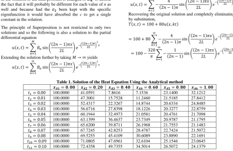
[image:3.595.52.530.174.484.2]
Table 1. Solution of the Heat Equation Using the Analytical method
100.0000 41.0591 7.8616 7.1536 23.1400 32.1212
100.0000 47.3001 15.7528 11.2460 21.5185 27.8412
100.0000 52.4317 22.3267 14.8744 20.6334 24.8485
100.0000 56.6716 27.8398 18.1226 20.3277 22.8759
100.0000 60.1944 32.4973 21.0581 20.4761 21.7098
100.0000 63.1399 36.4637 23.7349 20.9787 21.1795
100.0000 65.6200 39.8711 26.1968 21.7553 21.1483
100.0000 67.7245 42.8253 28.4787 22.7424 21.5072
100.0000 69.5255 45.4109 30.6089 23.8890 22.1691
Figure 1: A 3D-Plot of the data produced in the Analytical solution
6. NUMERICAL SOLUTION OF THE
HEAT EQUATION
To solve the heat equation numerically, both the x and t variables need to be discretized and proceed to deal with the x-variable employing finite difference approximation. This concept according to these great schools of thought Schmidt and Crank-Nicolson is presented in this paper.
6.1 Schmidt Scheme
When Dirichlet boundary conditions are imposed, those values must be specified at the boundary points. The first-order forward-time second-first-order centred-space (FTSC) approximation of the heat equation is given by
6.1.1
Stability of Schmidt Scheme Using Von
Neumann/Fourier Method
Let
(1)-(2)
Von Neumann considers the homogenous part of the difference equation
Using Fourier series, the n-component solution of the difference scheme is
Substituting (4) in (3) and simplifying yields
With the following trigonometric identities
Equation (5) then becomes
For the original error not to grow, the amplification factor is
restricted as
As sine function has the range
But
This confirms that provided then the Schmidt scheme will be stable, otherwise it will be unstable. In other words, the Schmidt scheme is conditionally stable.
For the purpose of this paper, r is set to 0.5 to achieve stability. The table below shows the resulting computations using the Schmidt scheme.
1
2
3 4
5
6
0 5
10 15
0 20 40 60 80 100
x t
u
Time t (sec) Temperature
T (x, t) oC
Displacement x (ft) Time t (sec)
Temperature
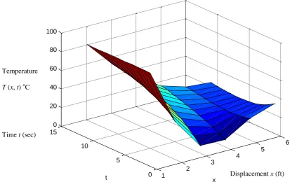
Table 2. Solution of the Heat Equation using the Schmidt Scheme
100.0000 20.0000 20.0000 20.0000 20.0000 20.0000 100.0000 40.0000 20.0000 20.0000 20.0000 20.0000 100.0000 50.0000 25.0000 20.0000 20.0000 20.0000 100.0000 56.2500 30.0000 21.2500 20.0000 20.0000 100.0000 60.6250 34.3750 23.1250 20.3125 20.0000 100.0000 63.9063 38.1250 25.2344 20.9375 20.0000 100.0000 66.4844 41.3477 27.3828 21.7773 20.0000 100.0000 68.5791 44.1406 29.4727 22.7344 20.0000 100.0000 70.3247 46.5833 31.4551 23.7354 20.0000
[image:5.595.104.486.259.522.2]100.0000 71.8082 48.7366 33.3072 24.7314 20.0000 100.0000 73.0882 50.6471 35.0206 25.6925 20.0000
Figure 2: A 3D-Plot of the data produced by the Schmidt scheme with r=0.5
6.2
Cranch Nicolson Scheme
6.2.1
Stability Analysis of the Crank-Nicolson
Scheme Using Von Neumann/Fourier Method
Let
Using Fourier series, the n-component solution of the difference scheme is
Substituting (d) in (c) and simplifying yields
With the following trigonometric identities
Equation (f) then becomes
Guided by the fact that and
1
2
3 4
5
6
0 5
10 15
20 40 60 80 100
x t
u
Temperature
T (x, t) oC
Time t (sec)
[image:6.595.43.516.146.289.2]
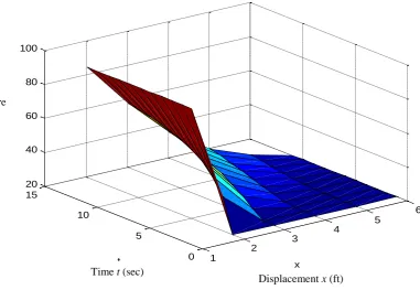
This shows that the Crank-Nicolson scheme is unconditionally stable but for the sake of uniformity and comparison, is chosen. The result of the Crank-Nicolson scheme computation is shown in the table below:
Table 3. Solution of the Heat Equation Using the Crank-Nicolson Scheme
100.0000 20.0000 20.0000 20.0000 20.0000 0.0000 100.0000 36.1612 21.6122 19.9608 17.9961 20.0000 100.0000 46.3832 25.2524 20.3454 18.8283 20.0000 100.0000 53.2854 29.3022 21.4936 19.4809 20.0000 100.0000 58.2207 33.1921 23.1086 20.1487 20.0000 100.0000 61.9253 36.737 24.9626 20.8964 20.0000 100.0000 64.8192 39.9033 26.9036 21.7244 20.0000 100.0000 67.1532 42.7133 28.8372 22.6087 20.0000 100.0000 69.0838 45.2061 30.7071 23.5197 20.0000
100.0000 70.7131 47.4223 32.4821 24.4307 20.0000 100.0000 72.1100 49.3985 34.1466 25.3213 20.0000
Figure 3: A 3D-Plot of the data produced in the Crank-Nicolson scheme with r = 0.5. 1
2
3
4 5
6
0 5
10 15
0 20 40 60 80 100
x t
u
Displacement x (ft) Time t (sec)
Temperature
[image:6.595.101.483.319.598.2]7.
DATA ANALYSIS
Table 4. Relative Errors in Numerical Approximations Using the Schmidt Scheme
0.0000 0.5129 1.5440 1.7958 0.1357 0.3774
0.0000 0.1543 0.2696 0.7784 0.0706 0.2816
0.0000 0.0464 0.1197 0.3446 0.0307 0.1951
0.0000 0.0074 0.0776 0.1726 0.0161 0.1257
0.0000 0.0072 0.0578 0.0982 0.0080 0.0788
0.0000 0.0121 0.0456 0.0632 0.0020 0.0557
0.0000 0.0132 0.0370 0.0453 0.0010 0.0543
0.0000 0.0126 0.0307 0.0349 0.0004 0.0701
0.0000 0.0115 0.0258 0.0276 0.0064 0.0978
0.0000 0.0102 0.0218 0.0214 0.0168 0.1329
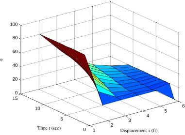
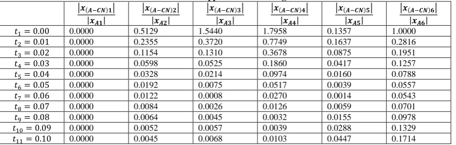
[image:7.595.67.534.611.760.2]0.0000 0.0090 0.0183 0.0150 0.0307 0.1714
Figure 4: A 3D-Plot of the absolute relative error with the Schmidt scheme
Table 5. Relative Errors in Numerical Approximations Using the Crank-Nicolson Scheme
0.0000 0.5129 1.5440 1.7958 0.1357 1.0000
0.0000 0.2355 0.3720 0.7749 0.1637 0.2816
0.0000 0.1154 0.1310 0.3678 0.0875 0.1951
0.0000 0.0598 0.0525 0.1860 0.0417 0.1257
0.0000 0.0328 0.0214 0.0974 0.0160 0.0788
0.0000 0.0192 0.0075 0.0517 0.0039 0.0557
0.0000 0.0122 0.0008 0.0270 0.0014 0.0543
0.0000 0.0084 0.0026 0.0126 0.0059 0.0701
0.0000 0.0064 0.0045 0.0032 0.0155 0.0978
0.0000 0.0052 0.0057 0.0039 0.0288 0.1329
0.0000 0.0045 0.0068 0.0103 0.0447 0.1714
1
2
3
4
5
6
0 5
10 15
0 0.5 1 1.5 2
x t
u
Displacement x (ft) Time t (sec)
Temperature
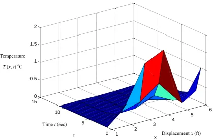
Figure 5: A 3D Plot of the Absolute Relative Error with the Crank-Nicolson scheme.
8. DISCUSSION OF RESULTS
For an aluminium rod at room temperature whose one end is insulated and the other immersed in boiling water, one would expect that with time the temperature will grow uniformly through the rod until such a time that the temperature distribution is the same across the whole rod. Even though, the rod was not given enough time to undergo such a transformation, that is, with in a time span of ,it was still evidently clear that the temperature distribution was actually growing across the rod.
For the analytical solution, the temperature distribution at
, for , fell below the room temperature of the rod, which was quite unusual. It begun to improve when , and only at when temperature actually fell below room temperature. For
and something unusual was happening. All the temperature at that point was actually less than the insulated end of the rod.
The aluminium rod begun to exhibit its true conductivity characteristics from , when there was truly uniformity in heat transfer.
The Schmidt scheme conforms to initial conditions of the rod perfectly. Heat only begins to flow at when the
temperature doubled at the point while other parts of the rod remained at room temperature. The temperature gradually increases through the rod until when all parts of the rod had experience temperature rise. This time conforms to the time the rod exhibits its conductivity properties.
The initial conditions of the rod is perfectly obeyed by the Crank-Nicolson method with the exception that . This defeats the fact that . This initial condition is however satisfied from whiles experiences a decrease in temperature. This negative phenomenon decreases in the range . The conductivity property of the rod then starts from .
Generally, the values obtained with the Schmidt and the Crank-Nicolson schemes compare favourably with values obtained with the analytical method of solution
. The true value for the final solution for the Analytical, Schmidt, and Crank-Nicolson schemes is shown in Table 6;
1
2
3
4
5
6
0 5
10 15
0 0.5 1 1.5 2
x t
u
Displacement x (ft) Time t (sec)
Temperature
Table 6. True Values of the Various Methods to the Heat Equatio
The above table clearly shows how close the numerical solutions with both the Schmidt scheme and the Crank-Nicolson scheme are to the Analytical solution. Shear
observation of the above table shows which numerical scheme is closer to the analytical scheme. But the best guide is the result from the absolute relative errors of the two numerical schemes, which is shown in table 7.
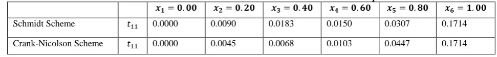
Table 7. Absolute Relative Error for the Final Solution of the Heat Equation.
Schmidt Scheme 0.0000 0.0090 0.0183 0.0150 0.0307 0.1714
Crank-Nicolson Scheme 0.0000 0.0045 0.0068 0.0103 0.0447 0.1714
Both schemes’ absolute relative error at the boundary points, that is, and are the same. In the range
, the Crank-Nicolson scheme is the best representation of the Analytical solution. However for , the Schmidt scheme seems to perform better than the Crank-Nicolson scheme.
However on a scale of 100, the Crank-Nicolson scheme will occupy 75 while the Schmidt scheme will occupy 25. This alone cannot however inform the choice of one over the other because if one considers a particular point alone on the rod, the Schmidt may be better than the Crank-Nicolson scheme.
9. CONCLUSIONS
At all discrete points of the rod at the given time frame , the analytical solution fails to conform to the initial conditions of the problem. This is so because the temperature of the rod at the insulated end at time
is supposed to be whiles the remaining points were supposed to be very close to the initial temperature with the exception of the end immersed in boiling water.
Ironically, the temperature at point was somehow closer to the room temperature than at the point
. This is surprising since heat transferred from the immersed end of the rod actually reduces as it gets to the insulated end. The analytical method however suggests that within the range temperature was rising instead of falling. There was however exception for the time frame at points on the rod where the behaviour conducting property of the rod was obeyed.
The Schmidt scheme obeys and conforms perfectly with the initial conditions of the rod, maintaining the initial temperature of at all points of the rod with the exception of the immersed end which assumes the temperature of the boiling water. This presents the Schmidt scheme as a huge improvement of the analytical method.
The Crank-Nicolson scheme complies well with the initial conditions except at the boundary when it is supposed to be
but the numerical solution actually gives . Per the Analytical method, the rod’s conductivity drops in the range for the time before it rises again. For the Crank-Nicolson scheme, the anomaly in heat conduction is seen at in the time interval where as the Schmidt scheme had no anomaly.
With r specially chosen such that the stability of both the Schmidt and Crank-Nicolson schemes is not compromised, the claim of superiority of one scheme over the other is far fetched. Infact superiority can only be claimed with respect to a particular discrete point in question.
The Schmidt scheme has shown to be more reliable than the Crank-Nicolson scheme which is strangely seen as an improvement of the Schmidt scheme.
10. REFERENCES
[1] Glenn Ledder. 2005. Differential Equations: A Modeling Approach. McGraw-Hill.
[2] John H. Matthews and Kurtis D. Fink 2004. Numerical Methods Using MATLAB. Pearson Education, Inc.
[3] Paul Dawkins. 2007. Lecture Notes on Differential Equations. http://tutorial.math.lamar.edu.
[4] David Richards and Adam Abrahamsen. 2002. The One Dimensional Heat Equation.
[5] Alfio Quarteroni, Riccardo Sacco and Fausto Saleri. 2000. Numerical Mathematics. Springer-Verlag New York, Inc.
[6] Golub, Gene H., and James M. Ortega. 1992. Scientific Computing and Differential Equation: An Introduction to Numerical Methods. San Diego: Academic Press.
Analytical Scheme 100.0000 72.4358 49.7355 34.5014 26.5072 24.1379
Schmidt Scheme 100.0000 73.0882 50.6471 35.0206 25.6925 20.0000
[image:9.595.52.538.218.274.2]