http://dx.doi.org/10.4236/alamt.2015.53010
A Real-Time Transient Analysis of a
Functionally Graded Material Plate
Using Reduced-Basis Methods
Yonghui Huang1, Yi Huang2
1Sunwoda Electronic Co., Ltd., Guangdong, China
2College of Mechanical and Vehicle Engineering, Hunan University, Changsha, China
Email: [email protected]
Received 28 July 2015; accepted 4 September 2015; published 7 September 2015
Copyright © 2015 by authors and Scientific Research Publishing Inc.
This work is licensed under the Creative Commons Attribution International License (CC BY).
http://creativecommons.org/licenses/by/4.0/
Abstract
Based on the hybrid numerical method (HNM) combining with a reduced-basis method (RBM), the real-time transient response of a functionally graded material (FGM) plates is obtained. The large eigenvalue problem in wavenumber domain has been solved through real-time off-line/on-line calculation. At off-line stage, a reduced-basis space is constructed in sample wavenumbers according to the solved eigenvalue problems. The matrices independent of parameters are projected onto the reduced-basis spaces. At on-line stage, the reduced eigenvalue problems of the arbitrary wa-venumbers are built. Subsequently, the responses in wavenumber domain are obtained by the approximated eigen-pairs. Because of the application of RBM, the computational cost of transient displacement analysis of FGM plate is decreased significantly, while the accuracy of the solution and the physics of the structure are still retained. The efficiency and validity of the proposed me-thod are demonstrated through a numerical example.
Keywords
Reduced-Basis Method, Transient Response, Functionally Graded Material, Hybrid Numerical Method, Real-Time
1. Introduction
significant-ly the size of the problem and the computational cost but also retain the accuracy of the solution and the physics of the structures are very desirable.
Many methods on model-order reduction, such as Guyan reduction [1], Ritz vectors reduction [2], proper or-thogonal decomposition [3], balanced truncation [4], and various related hybrid techniques [5] [6], have been developed to reduce the problem size of structures. Recently, there has been considerable interest in the re-duced-basis method (RBM) [7]-[10], a very promising numerical method, which requires a projection onto the reduced-basis space constructed by the solutions of the interest sample parameter points, which is very suitable for the analysis of large system. The RBM has first been introduced in the late 1970s for single-parameter prob-lems in nonlinear structural analysis and subsequently developed for multi-parameter probprob-lems. However, RBM has rarely been extended to the real-time analysis of the dynamic problems yet, especially the transient analysis of large complex structures.
Hybrid numerical method (HNM) which combines the finite element method with the Fourier transform, a very efficient method to perform the transient analysis of laminated structures, is proposed by Liu etal [11]. Later the modified HNM [12] [13] is developed to analyze the associated characteristics of functionally graded material (FGM) structures. In the modified HNM, the structures are firstly divided into inhomogeneous layered elements in one direction. A set of partial differential equations (PDEs) is developed to approximate the dynam-ic equilibrium of the FGM structures by applying the principle of virtual work and assembling the matrdynam-ices of adjacent elements. The PDEs are solved effectively through a space-wavenumber Fourier transform. However, the repeated calculations of eigenvalue problems in wavenumber domain are very expensive, especially in the three-dimensional case where structures are subjected to a point load.
In this paper we apply the reduced-basis method in wavenumber domain to the transient analysis of structures based on the modified HNM. The truncated eigenvectors corresponding to the carefully selected sample para-meter points are extracted to construct the reduced-basis space onto which the original large system problem is projected. In this manner, a reduced system is obtained and the eigenvalue problem can be solved more effec-tively. And then the eigenvectors of the full problem are obtained by the inverse projection; the response in wa-venumber domain can be obtained by a real-time manner. Eventually the transient response in space-time do-main is obtained through performing the inverse Fourier transform.
2. Brief Introduction of the Modified HNM to FGM Plate
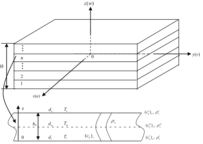
A functionally graded material (FGM) plate with varying material properties in the thickness direction as shown
in Figure 1 is considered. The plate is composed of two materials and divided into N layered element in the
thickness direction. Without losing the generality, the elastic modulus matrix of an element possesses 21 differ-ent constants. H is the thickness of the plate and hn is the thickness of the nth element. The displacement field,
elastic constants and mass density of the nth element are approximated as [13]:
d
=
U N d (1)
( )
cij n=N cp( )
ij′ n(
i j, =1, ,6)
(2)p
n =N n′
ρ ρ (3) where Nd and Np are the shape function matrices of the second-order interpolations. d denotes the nodal
displacement vector, which are functions of x, y and time t, at z=0, z=0.5hn and z h= n, as following:
{
}
T T T T
l m u
=
d d d d (4)
where
{
}
(
)
T , ,
i = d d dx y z i i l m u=
d (5)
( )
{
( ) ( ) ( )
l m u}
Tij′ n = ij n ij n ij n
c c c c ,
{
l m u}
n′ = ρn ρn ρn
ρ (6)
0 1 2
0 n
H
z
hn
( )cij n
n
ρ
( ) ,u u
ij n n
c ρ
( ) ,l l
ij n n
c ρ
( ) ,m m
ij n n
c ρ
u
T
u
d
m
T
l
T
m
d
l
d
( ) z w
( )
y v
( )
[image:3.595.140.487.86.332.2]x u
Figure 1. A functionally graded material plate and the nth isolated layered element.
0 , 0
t= = t= =
d 0 d 0 (7) d is the transient displacement responses vector of the nodal planes and “.” denotes the differentiation with respect to time t.
With the principle of virtual work, a set of approximate partial differential equations for an element is ob-tained. The dynamic equilibrium equation of the whole plate can be formed by assembling the matrices of all the adjacent elements. The Fourier transform from space to wavenumber is used to deduce a set of system equations of the FGM plate in wavenumber domain [13].
F = Md + Kd (8) where F, d, and d are the Fourier transform of load, acceleration, and displacement, respectively. Hermi-tian stiffness matrix K is given by
(
)
2 21 2 3 4 5 6
, i i
x y x x y y x y
k k =k +k k +k − k − k +
K A A A A A A (9)
which is constant matrix for the given wavenumbers kx and ky. The expressions of the matrices Ai
(
i=1,2, ,6)
and mass matrix M can refer to [13]. The dimension of the stiffness and mass matrices is(
)
3 2N 1
= +
3. The Introduce of RBM into the Modified HNM
An alternative expression of Equation (8) can be obtained through rearranging columns and rows in the matrices by degrees of freedom rather than by interface. The resulting representation is given by
1 2 3 4
2 2
1 2 3 4
1 2 3 4
5 6
2
5 6
5 6
i
i
x x x x x
y y x y x y y x y x
z z z z z
x x x x
y y y y y
z z z z
k k k k k
k ω
= + + +
+ + −
F A A A A
F A A A A
F A A A A
A A M d
A A M d
A A M d
where Aix= Aixx Aixy Aixz, Aiy = Aixy Aiyy Aiyz, Aiz = Aixz Aiyz Aizz (i = 1, 2, 3, 6).
jx = jxx jxy jxz
A A A A , T
jx= − jxy jyy jyz
A A A A , T T
jx = − jxz − jyz jzz
A A A A (j = 4, 5).
In the particular case where the elastic material possesses a symmetric plane, multiplying the third row of Equation (10) by i= −1 and factoring out i from the third column, the stiffness matrix K can be turned to a real symmetrical one and expressed as follows.
( )
6( )
1 i i
i
µ σ µ
=
=
∑
K A (11)
where µ includes the two parameters ,k kx y. The displacement d can be evaluated through the modal
su-perposition using the conjugated eigenvectors of the generalized eigenvalue equation:
( )
µ ω2 0 − =
K MΦ (12)
The above equation can be converted to standard form by performing Cholesky decomposition of mass matrix.
T
=
M U U.
( )
µ =λQ X X (13) where Q
( )
µ is the characteristic matrix.( )
6( )
1 i i
i
µ σ µ
=
=
∑
Q B, T
i = i
B U AU (14)
It requires the repeated analysis of eigenvalue problem in wavenumber domain. When the inverse Fourier transform is performed, the range of integration is theoretically from negative infinite to positive infinite wave-numbers. For a practical calculation, the ranges of wavenumbers and the number of sampling points should be chosen properly according to the required accuracy before Fourier transform. Generally, hundreds of sample points in wavenumber domain are required to guarantee the accuracy of results. Nevertheless, the eigenvalue problem for individual wavenumber should be solved to perform the modal superposition before the inverse Fourier transform, this is computationally expensive. Furthermore, for higher accuracy of results, the computa-tional cost will increase exponentially when layered element is adopted.
The expensive computational cost of the repeated analysis for the large eigenvalue problems can be decreased by reduced-basis method through an off-line/on-line decomposition [14] [15]. Figure 2 provides the procedure of the real-time analysis of the transient response.
At off-line stage, we introduce a sample set SG=
{
µ1, , µG m}
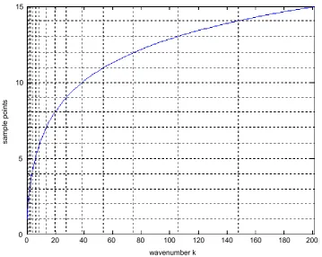
in the wavenumber domain, assuming G can be exactly divided by m. m denotes the number of truncated eigenvectors from Equation (13) associated with the desired accuracy of calculation. The sample points are logarithmically distributed in the sense that [15]:(
)
1(
max) (
)
ln 1 ln 1 1, ,
1
g g
ak ak g G
G −
+ = + =
− (15)
where G is the number of the sample point, kmax denotes the maximum wavenumber, a is a constant to
guarantee the relationship between the serial number of the sample points and the value of the corresponding wavenumber. Figure 3 gives the logarithmically distribution of the sample points. For each input in SG, we
solve the standard eigenvalue problem Equation (13).
A reduced-basis space can be introduced by extracting the first m eigenvectors of each point in the sample set as follows [8]:
( )
( )
( )
( )
( )
( )
{
1 1 , , 1 , 1 2 , , 2 , , 1 , ,}
G
m m G m m G m
W =span X µ X µ X µ X µ X µ X µ (16)
To simplify the notation, we rewrite Equation (16) as follows:
{
1, , ,2}
G
G
Selection of sample set in wavenumber domain
Piecewise approximation
Solve the associated eigenvalue problems
Construct the reduced eigenvalue problem and
explore the whole wavenumber domain
Regenerate the eigenvectors
Perform the modal superposition to obtain
the response in wavenumber domain
Perform the inverse Fourier transform to obtain the response in
space-time domain Construct reduced-basis
spaces using the truncated eigenvectors
Project the parameter independent matrices to the reduced-basis spaces
[image:5.595.121.527.81.406.2]Off-line stage On-line stage
Figure 2. Off-line/on-line decomposition procedure of transient analysis.
0 20 40 60 80 100 120 140 160 180 200
wavenumber k 0
5 10 15
sam
pl
e poi
nt
s
[image:5.595.134.494.409.695.2]Galerkin projection:
(
)
1
ˆj G ij i 1,2, ,
i j m
α =
=
∑
=X η (18)
where the subscript j denotes the jth mode, ‘^’ denotes the approximated variable. It can also be rewritten in the
form of a matrix.
(
)
ˆj = j j=1,2, ,m
X Zα (19)
where Z=
(
η η1, , ,2ηG)
is a n G× matrix, and αj is the generalized coordinates column.The matrices independent of wavenumber are projected onto the reduced-basis space:
(
)
T 1, ,6
G
i = i i=
B Z B Z (20)
At on-line stage, because of the wavenumber independence of G i
B , we can form the reduced-basis characte-ristic matrix and explore the whole wavenumber domain easily.
( )
6( )
1
G G
i i
i
µ σ µ
=
=
∑
Q B (21)
The resultant reduced eigenvalue problem can be expressed as:
( )
ˆG µ =λ
Q α α (22) where α =
(
α1, ,αm)
. The truncated eigenvectors of the original large system for arbitrary µ can berege-nerated using the following equation.
( )
1 ˆ( )
1ˆ − −
= U X = U Zα
Φ (23)
Combining the method of modal analysis, the initial condition Equation (7) with the addition of the Duhamel integral, the displacements in Fourier transform domain can be obtained.
Finally, the approximate displacement response in the space-time domain can be obtained by performing the inverse Fourier transform.
It is considerable for the reduced standard eigenvalue problem that the reduced-basis space which is con-structed by the truncated modes can only approximate the same modes of the eigenvalue problem for a new µ. The size of the reduced system equation is independent of the original system, it depends on the required accu-racy and the selected sample set.
4. The Error Bound of Approximated Eigen-Pairs
According to the classical theory of matrix projection, the following equation holds if Z is an invariant subspace for matrix Q.
( )
( )
( )
( )
3 3 3 3
T
1 1 1 1
N
i i i G i i i i i
i k i k i k i k
σ σ σ σ
= = = =
=
∑
=∑
=∑
≈∑
QZ B Z P B Z ZZ B Z ZB
Here T
G=
P ZZ is an orthogonal projection matrix. However, an error will be introduced for an approx-imated subspace.
( )
3
1
N
i i
i k
σ =
=
∑
+QZ ZB E
E denotes the deviation matrix of the approximated subspace within invariant subspace, which can be ex-pressed as:
[
1]
3( )
1
N
N i i i
i k
σ =
= =
∑
− E θθ B Z ZB
2 2 1
N i E
i=
=
∑
E θ
It is easy to guarantee the error within bound of eigenvalue. ˆ
i i E
λ λ− ≤ E
The error of eigenvectors is also bounded.
5. Results and Discussions
The present method is applied to an actual stainless steel-silicon nitride (SS-SN) FGM plate, in which the silicon nitride is considered as the inclusion material. The material constants for SS-SN are listed in Table 1[16]. The volume fraction of SN is assumed as the following simple power law distribution in the thickness direction:
(
)
2(
)
0.5 2 2
V = +z H −H ≤ ≤z H (24) The material property of the FGM can be obtained by using the rule-of-mixture [16]. The whole plate is di-vided into 10 layered elements and has 63 degrees of freedom.
In the computational procedure, the following dimensionless parameters are used [13].
0 0 0 0 0 0 0 0 0
2 2
0 0
, , , ,
, , , ,
t t t t H c c G u u u u q G w w u H c x x H z z H k kH
ρ λ λ
= = = = =
= = = = = (25)
For the SS-SN FGM plate, the SS material is taken as the referenced material, ρ0, G0, c0 and t0 are the
mass density, the shear modulus, the velocity of shear wave in SS material and the time for the shear wave to cross the plate thickness, respectively.
Consider two-dimensional case, a vertical line sin load is acted on the upper surface at x0=0:
( ) ( )
0F t δ x =
F P (26)
where
( )
sinπ , 0 2.0 0, 0 and 2.0t t
F t
t t
< <
= ≤ ≥
(27)
{
}
T= 0,0, ,0, ,0−q
P (28)
Equation (26) implies that the time history of the load is only one cycle of the sin function, P is a constant amplitude vector and q is a constant. The observation position is at x=10.0H on the upper surface of the plate.
In this case where ky =0 and kx should only be taken into account. The range of wavenumber [0, 64π] is
[image:7.595.119.510.658.717.2]divided into 751 points, the sub domains are cut by some prescribed sample points. Due to the well behavior of dispersion in wavenumber domain, we adopt a piecewise approximation. And the eigenvectors are only from two external points used to construct the reduced-basis space in each sub domain. In the two-dimensional tran-sient analysis of structures, the first six eigenvectors are only needed to perform the modal superposition. The reason is that it needs only the first several natural modes to perform the modal superposition in practice, while the effect of the high order modes on the result is little. Therefore, the truncated eigenvectors from the two sam-ple points are extracted to construct a reduced-basis space of 12 basis vectors in each sub domain. The original large eigenvalue problem can be reduced to 12 12× by projection.
Table 1. Material constants of stainless steel and silicon nitride monolith [13].
Material E (GPa) ν ρ(kg/m3)
Stainless steel 207.82 0.3177 8166
The eigen-pairs analysis in six wavenumbers, namely k1=0.37699, k2 =0.62832, k3=1.82210, 4 2.51330
k = , k5 =4.39820 and k6 =6.28320 are applied to validate the present reduced-basis method when
[image:8.595.94.538.194.446.2]15 sample points are selected. As comparison, the error of eigenvalues is listed in Table 2, and the norm error of eigenvectors is listed inTable 3. The biggest error of eigenvalues from RBM is 0.69706%, and RBM almost exactly regenerates the eigen-pairs in the second and the forth mode. The other eigen-pairs from RBM are also agreement with that from HNM without the introducing of RBM very well. The RBM simulation can obtain the sufficient accuracy for the practical engineering and the high reliability for the numerical calculation.
Table 2. The error of the first six eigenvalues from RBM with respect to that without RBM at six wavenumbers (%).
k Modal
1 2 3 4 5 6
1 EERBMori
deviation 0.0015476 0.0015584 (0.69706%) 0.053833 0.053833 (0%) 0.136998 0.137009 (0.00823%) 3.994015 3.994015 (0%) 4.123671 4.123691 (0.00049%) 10.856721 10.857459 (0.00680%)
2 EERBMori
Deviation 0.0110826 0.0110911 (0.07657%) 0.148887 0.148887 (0%) 0.376779 0.376789 (0.00263%) 4.107236 4.107236 (0%) 4.461153 4.461169 (0.000367%) 10.659006 10.659572 (0.005308%)
3 EERBMori
Deviation 0.445148 0.445160 (0.00276%) 1.194321 1.194321 (0%) 2.840223 2.840235 (0.00041%) 5.451391 5.451391 (0%) 7.8919523 7.8920416 (0.00113%) 10.320135 10.320669 (0.00518%)
4 EERBMori
Deviation 1.136406 1.136437 (0.00529%) 2.178978 2.178978 (0%) 4.884445 4.884461 (0.00068%) 6.871678 6.871678 (0%) 9.501102 9.501483 (0.008%) 12.827217 12.827740 (0.00764%)
5 EERBMori
Deviation 4.512785 4.512792 (0.00276%) 5.954376 5.934376 (0%) 10.541770 10.541834 (0.00034%) 13.050998 13.050998 (0%) 15.398164 15.398204 (0.00401%) 23.799351 23.799351 (0%)
6 EERBMori
Deviation 9.046870 9.046886 (0.00019%) 11.155957 11.155957 (0%) 18.462705 18.462744 (0.00022%) 21.648815 21.648816 (0%) 25.946279 25.946399 (0.00046%) 33.442165 33.442174 (2.7e-005%)
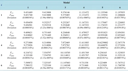
Table 3. The error norm of the first six eigenvectors from RBM with respect to that without RBM at six wavenumbers (%).
k Modal
1 2 3 4 5 6
1 FFRBMori
Deviation 9.451689 9.451740 (0.00054%) 9.413008 9.413008 (1.94e-006%) 9.376146 9.375485 (0.00705%) 11.131472 11.131472 (3.61e-006%) 11.135540 11.133934 (0.01443%) 11.197055 11.200604 (0.03170%)
2 FFRBMori
Deviation 9.456450 9.456501 (0.00054%) 9.352517 9.352518 (3.23e-006%) 9.253267 9.252640 (0.00678%) 11.167351 11.167352 (6.09e-006%) 11.175687 11.174335 (0.01210%) 11.226883 11.231277 (0.03914%)
3 FFRBMori
Deviation 9.409621 9.410042 (0.00447%) 8.751445 8.751449 (3.52e-005%) 8.236840 8.236911 (0.00086%) 11.478927 11.478937 (8.07e-005%) 10.931823 10.939108 (0.06664%) 12.054381 12.053443 (0.00778%)
4 FFRBMori
Deviation 9.271804 9.273026 (0.01318%) 8.314886 8.314896 (0.00012%) 7.872469 7.872762 (0.00373%) 11.611885 11.611933 (0.00041%) 10.6239002 10.644070 (0.18985%) 12.367178 12.371036 (0.03120%)
5 FFRBMori
Deviation 8.334712 8.335180 (0.00561%) 7.554797 7.554795 (2.13e-005%) 10.118705 10.114811 (0.03848%) 11.051769 11.051787 (0.000164%) 9.256165 9.258184 (0.02181%) 11.525035 11.525118 (0.00073%)
6 FFRBMori
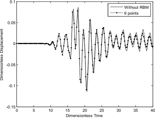
[image:8.595.90.537.473.723.2]Either too many or too few sample points selected in the parameter domain is unfeasible, the former leads to computational inefficiency, while the latter leads to unacceptable error. There is often a tradeoff between the computational cost and the accuracy of the simulated result. The transient displacements from RBM with 6, 8 and 15 sample points compared with that from HNM without the introducing of RBM are drawn in Figure 4 and
Figure 5 respectively. It can be seen from Figure 4 that the simulated result will be distorted if too few points of the sample set is selected, especially in the duration when loads are unloaded. Figure 5 shows that the results from RBM are agreement with that from HNM without using RBM very well. Fortunately, it can be found that the results from RBM become steady when the number of the sample points increases up to a critical number 8, as let us avoid dealing with the tradeoff.
[image:9.595.165.461.467.695.2]Figure 4. Comparison of the response of time history on the upper surface (with 6 sample points or without RBM).
Figure 5. Comparison of the response of time history on the upper surface (with 8, 15 sample points or without RBM).
0 5 10 15 20 25 30 35 40
-0.15 -0.1 -0.05 0 0.05 0.1
Dimensionless Time
D
im
ens
ionl
es
s D
is
pl
ac
em
ent
Without RBM 6 points
0 5 10 15 20 25 30 35 40
-0.15 -0.1 -0.05 0 0.05 0.1
Dimensionless Time
D
im
ens
ionl
es
s D
is
pl
ac
em
ent
Table 4. Computational costs for the analysis of eigenvalue problems with or without the in-troduce of RBM.
CPU time (s) With RBM Without RBM
1.625 4.188
The Fortran codes for the calculation of transient displacements are executed on a PC with a CPU clock speed of 2.8 GHz. The CPU time for the analysis of eigenvalue problems with and without the introducing of RBM are compared in Table 4 and it can be found that time of the former is about 38.8% of the later. It is mainly reason that the efficient off-line/on-line decomposition is used. In addition, the projection of the original eigenvalue problem onto the reduced-basis spaces is just a procedure to perform multiplication of several matrices, as costs very little CPU time. The efficiency can be further enhanced when the layered element refined for higher accuracy. For a practical dynamic analysis of complex structures, the number of degree-of-freedom is typically extremely large, and in particular much too large to perform transient response analysis. Fortunately, the size of the system equations projected onto the reduced-basis space is independent of the original system rather decided by the di-mensions of the reduced-basis space. No matter how large the system structure is, it always can be reduced to a small size by reduced-basis method while the physics of the original structures are retained, as ensure us to per-form the accurate transient response analysis by a real-time manner.
6. Conclusion
A reduced-basis method in wavenumber domain is proposed to obtain the real-time transient response of FGM plate based on the modified HNM in this paper. The repeated and expensive numerical analyzes of the large ei-genvalue problems have been simplified by RBM. Through a real-time off-line/on-line decomposition technique, high accuracy and less cost of the simulation are achieved. Because of the outstanding performance of the RBM, it is a promising numerical method which can be extended to the dynamic analysis of other complex structures.
Acknowledgements
This project is supported by National Natural Science Foundation of China (Grant No. 51305045), and by China Postdoctoral Science Foundation (No. 2014M562099).
References
[1] Guyan, R.J. (1965) Reduction of Stiffness and Mass Matrices. AIAA Journal, 3, 380-381.
http://dx.doi.org/10.2514/3.2874
[2] Wilson, E.L. and Bayo, E.P. (1967) Use of Special Ritz Vectors in Dynamic Substructure Analysis. AIAA Journal, 5, 1944-1954.
[3] Sirovich, L. and Kirby, M. (1987) Low-Dimensional Procedure for the Characterization of Human Faces. Journalof theOpticalSocietyofAmericaA, 4, 519-524. http://dx.doi.org/10.1364/JOSAA.4.000519
[4] Moore, B.C. (1981) Principal Component Analysis in Linear Systems: Controllability, Observability, and Model Re-duction. IEEETransactionsonAutomaticControl, 26, 17-32. http://dx.doi.org/10.1109/TAC.1981.1102568
[5] Lall, S., Marsden, J.E. and Glavaski, S. (2002) A Subspace Approach to Balanced Truncation for Model Reduction of Nonlinear Control Systems. International Journal of Robust and Nonlinear Control, 12, 519-535.
http://dx.doi.org/10.1002/rnc.657
[6] Willcox, K. and Peraire, J. (2002) Balanced Model Reduction via the Proper Orthogonal Decomposition. AIAA Journal, 40, 2323-2330. http://dx.doi.org/10.2514/2.1570
[7] McGowan, D.M. and Bostic, S.W. (1993) Comparison of Advanced Reduced-Basis Methods for Transient Structural Analysis. AIAA Journal, 31, 1712-1719. http://dx.doi.org/10.2514/3.11834
[8] Machiels, L., Maday, Y., Oliveira, I.B., Patera, A.T. and Rovas, D.V. (2000) Output Bounds for Reduced-Basis Ap-proximations of Symmetric Positive Definite Eigenvalue Problems. Comptes Rendus de l’Académie des Sciences—Series I, 331, 152-158.
[9] Ito, K. and Ravindran, S.S. (1997) Reduced Order Methods for Nonlinear Infinite Dimensional Control Systems. Pro-ceedingsofthe 36thConferenceonDecision&Control, San Diego, 10-12 December 1997, 2213-2218.
[10] Maday, Y., Patera, A.T. and Peraire, J. (1999) A General Formulation for a Posteriori Bounds for Output Functionals of Partial Differential Equations; Application to the Eigenvalue Problem. Comptes Rendus de l’Académie des Sci- ences—Series I, 328, 823-828.
[11] Liu, G.R. and Xi, Z.C. (2002) Elastic Waves in Anisotropic Laminates. CRC Press, Boca Raton.
[12] Liu, G.R., Han, X., Xu, Y.G. and Lam, K.Y. (2001) Material Characterization of FGM Plates Using Elastic Waves and an Inverse Procedure. JournalofCompositeMaterials, 11, 954-971.
http://dx.doi.org/10.1106/86AQ-JY72-5VKT-K1NV
[13] Han, X., Liu, G.R., Xi, Z.C. and Lam, K.Y. (2001) Transient Waves in Plates of Functionally Graded Materials. Inter-national Journal for Numerical Methods in Engineering, 52, 851-865. http://dx.doi.org/10.1002/nme.237
[14] Veroy, K., Prud’homme, C. and Patera, A.T. (2003) Reduced-Basis Approximation of the Viscous Burgers Equation: Rigorous a Posteriori Error Bounds. Comptes Rendus de l’Académie des Sciences—Series I, 337, 619-624.
[15] Maday, Y., Patera, A.T. and Turinici, G. (2002) A Prior Convergence Theory for Reduced-Basis Approximations of Sing-Parameter Elliptic Partial Differential Equations. JournalofScientificComputing, 17, 437-446.
http://dx.doi.org/10.1023/A:1015145924517
[16] Touloukian, Y.S. (1967) Thermo-Physical Properties of High Temperature Solid Materials. Macmillan, New York. [17] Liu, G.R. (1998) A Step-by-Step Method of Rule-of-Mixture of Fiber- and Particle-Reinforced Composite Materials.
![Table 1. Material constants of stainless steel and silicon nitride monolith [13].](https://thumb-us.123doks.com/thumbv2/123dok_us/8073769.780342/7.595.119.510.658.717/table-material-constants-stainless-steel-silicon-nitride-monolith.webp)