Interpolating Value Functions in Discrete Choice Dynamic Programming Models

Munich Personal RePEc Archive

Interpolating Value Functions in Discrete

Choice Dynamic Programming Models

Sullivan, Paul

Bureau of Labor Statistics

October 2006

Online at

https://mpra.ub.uni-muenchen.de/864/

Interpolating Value Functions in Discrete Choice

Dynamic Programming Models

Paul Sullivan

Bureau of Labor Statistics

October 2006

Abstract

Structural discrete choice dynamic programming models have been shown to be a valuable tool for analyzing a wide range of economic behavior. A major limitation on the complexity and applicability of these models is the compu-tational burden associated with computing the high dimensional integrals that typically characterize an agent’s decision rules. This paper develops a regression based approach to interpolating value functions during the solution of dynamic programming models that alleviates this burden. This approach is suitable for use in models that incorporate unobserved state variables that are serially cor-related across time and corcor-related across choices within a time period. The key assumption is that one unobserved state variable, or error term, in the model is distributed extreme value. Additional error terms that allow for correlation between unobservables across time or across choices within a given time period may be freely incorporated in the model. Value functions are simulated at a fraction of the state space and interpolated at the remaining points using a new regression function based on the extreme value closed form solution for the expected maxima of the value function. This regression function is well suited for use in models with large choice sets and complicated error structures. The performance of the interpolation method appears to be excellent, and it greatly reduces the computational burden of estimating the parameters of a dynamic programming model.

1 In

tr

ct

In recent years a large amount of research has centered on the estimation of structural discrete choice

dynamic programming models of rational behavior. This type of model represents a theoretically

appealing approach to modelling situations in which a forward looking agent makes decisions in the

presence of uncertainty about future events. Existing research shows that dynamic programming

models are a valuable tool for examining a wide range of topics spanning many erent …elds of

economics such as industrial organization, labor, and development. Topics examined using dynamic

programming models include engine replacement (Rust 198 occupational choices (eane and

Wolpin ), retirement (Berkovec and Stern 1991, Rust and Phelan educational choices

(Arcidiacono 2004), and decisions about marriage and cohabitation (Brien, Lillard, and Stern 2006)

to name just a few examples.1

A major impediment to the estimation of dynamic discrete choice models is the computational

burden associated with solving the agent’s dynamic optimization problem. Solving the optimization

problem produces the value functions that are used to compute a likelihood function or set of

moment conditions that are used to estimate the parameters of the model. The value functions

must be computed for each feasible choice, in every time period, for every value of the state

variables that in‡uence choice-spec

…c rewards. Computing the value functions requires evaluating

the expected value of the maximum valued choice available in the next time period at each point

in the state space. In general, computing the expected value of the maximum choice, called Emax

in the remainder of this paper, involves computing a high dimensional integral. The computational

burden of solving a dynamic programming model grows rapidly as the size of the state space

increases, creating a well known problem known as the“curse of dimensionality (Bellman

Several approaches have been developed to reduce the computational burden of estimating

dynamic programming models. One approach takes advantage of particular functional form

sumptions and model structures so that evaluating high dimensional integrals is not required when

solving the dynamic programming problem (Miller 1984, Rust 19 For example, Rust

assumes that the only source of randomness in his model is an extreme value error term so that

Emax has a convenient closed form solution. A second approach reduces the computational burden

of estimation by estimating the parameters of a dynamic programming model without solving the

optimization problem (H and Miller 1993, Manski 1991). Aguirregabiria and Mira (2002) build

on this work and develop a method of estimating dynamic programming models that bridges the

gap between the full solution andH and Miller (1993) estimation approaches.

2 _{A third approach}

developed by Rust (199 solves the dynamic programming problem using a method that

circum-vents the curse of dimensionality using randomization. Finally,Keane and Wolpin (1994) develop

a method of approximately solving the dynamic programming problem that involves simulating

Emax at a fraction of the state space and then interpolating Emax at the remaining points in the

state space using a linear regression of Emax on the expected value functions for each choice. This

approach reduces computation time because it replaces relatively slow numerical integration with

comparatively fast interpolation.

This paper develops a method for solving dynamic programming problems that combines

fea-tures of the interpolation method developed by K and Wolpin (1994) with a less restrictive

version of the functional form assumptions used by Rust . The key assumption is that there

is one unobserved state variable, or error term, in the model that is distributed extreme value.

There are no restrictions on the other error terms in the model, so additional error terms that allow

for correlation across choices within a given time period or for correlation between error terms

across time may be freely incorporated. Allowing unobservables to be correlated across choices and

2_{One limitation of these non-full solution esitmation methods is that in general thay cannot be used when}

un-observable state variables are serially correlated. See Aguirregabiria and Mira (2006) for an estimation method for

across time is necessary in many natural applications of dynamic programming models in order to

develop economic models that are s ciently realistic to capture important aspects of behavior.

For example, any reasonable formulation of a job search model must allow for matching between

workers and rms, which requires formulating and solving a dynamic programming model that

incorporates serially correlated unobserved job match components. Similarly, in a dynamic model

whererms make entry decisions it is desirable to allow forrm spe c shocks to prtability that

are correlated across markets.3

Followinge !e and Wolpin (1994), the interpolation method developed in this paper involves

simulating the value functions at a subset of state points and interpolating the value functions

at the remaining points in the state space using a linear regression. The method departs from

e !e and Wolpin (1994) by using a new interpolating regression function that takes advantage

of the assumption that one of the error terms in the model is distributed extreme value.4 The

interpolating regression involves regressing Emax on a constant and the closed form solution that

Emax would take on if the only error term in the model was the extreme value error. The intuition

behind this regression function is that the"option value# arising from the non-extreme value error

terms is captured by the parameters of the interpolating regression. This regression function has

the desirable theoretical property that it converges to the exact solution for Emax as the standard

deviations of the non-extreme value error terms approach zero. In addition, the single regressor is

not vulnerable to the collinearity problems between regressors that can make it $ cult to apply

interpolating regressions that use individual expected value functions separately as explanatory

3_{In practice, only a very limited number of dynamic programming models that allow for serially correlated}

un-observed state variables have been estimated. See, for example, Pakes (1986), Berkovec and Stern (1991), Wolpin

(1992), and Stinebrickner (2001).

4_{Since the independence of irrelevant alternatives (IIA) problem is not present in dynamic programming models,}

the extreme value assumption has computational bene%ts analogous to those of estimating a multinomial logit model

variables. This problem is likely to arise in models with large choice sets and when several choices

have similar discounted expected values.

The interpolation method is tested using a dynamic structural model of occupational choices

and job search. This particular application of dynamic programming techniques is well suited to

examine the performance of the interpolating regression because it includes several features that

are likely to be found in a wide range of applications. For example, this model incorporates a large

choice set (21 choices) where the set of feasible choices varies over the state space. The model

also includes a large state space and a rich error structure that allows for correlation between

unobservable state variables both across choices within a given time period and across time for a

given choice.

The interpolation method is evaluated by examining the extent to which the interpolated value

functions generate choices that match the optimal choices produced by the model when the dynamic

program is solved exactly (without using interpolation). The performance of the interpolation

method is evaluated for three sets of structural parameters that create &' )erent lifecycle choice

patterns and also&' )er in the importance of the non-extreme value error terms. The performance of

the interpolation method is excellent, with at least 97 *of interpolated choices matching the optimal

choices across all three simulated data sets. The interpolation method is extremely accurate even

when the value functions are interpolated at99*of the state space. At this level of interpolation the

value functions can be computed over 100 times faster than when the value functions are computed

without using interpolation. The large decrease in computation time combined with the excellent

performance of the interpolation algorithm makes estimating dynamic programming models with

large choice sets, large state spaces, and complicated and realistic error structures computationally

feasible.

The remainder of the paper is organized in the following manner. Section 2 discusses the solution

of occupational choices and job search that is used to evaluate the performance of the interpolation

method. Section 4 presents evidence on the performance of the interpolating regression, and Section

5 concludes.

2 S+lv,-g D.-

a

c

scr

t

c

s

This section presents a dynamic programming model and discusses the solution to the agent’s

optimization problem. Assume that each individual chooses an action kt 3 Dt in each discrete

time period, t= 1; :::; T. Denote the number of elements in Dt asKt. Alternatives are de4ned to

be mutually exclusive. The individual’s objective is to choose the feasible alternative in each time

period that maximizes the discounted expected value of future rewards. The one period reward

from choosing alternative kin time period tis

Rt(k; St; kt; ekt; "kt) =Ut(k; St) + kt+ekt+"kt; (1)

where St is a vector of state variables that evolves deterministically over time conditional on the

chosen alternative, andUt(k; St) is a deterministic function of the state vector. The term kt is a

continuous random state variable thata5ects the reward from choosing alternativekin time period

t. This variable is constant over time as long as an individual chooses action k, so _{kt 1} = _kt if

kt 1 =kt. 6: 4ne the cumulative distribution function of

ktasG( ):The termektis a continuous

random state variable that may be correlated across the various alternatives within a time period

but is independent across time. 6 : 4ne the distribution of ekt asH(e). The variable "ktrepresents

a random shock to the reward from alternative k in time periodt that enters the reward function additively: Assume that "kt is independent across alternatives and across time, and is distributed

multivariate extreme value with variance 2 2_=6.

6: 4ne the cumulative distribution function of"kt

period realizations of these variables are observed by the agent when he makes his optimal choice

in each period.5

The agent’s optimization problem can be represented in terms of alternative sp; <= >c value

functions,Vt(k). ?;>ne the expected value of the individual’s optimal choice in time period t+ 1

for an individual who is currently in time period tas

EWt+1(St+1) = RRR max

fk2Dt+1g

fVt+1(k); k@Dt+1AdG( )dH(e)dF(") (2)

When computing the expected value of the optimal choice in the next time period the agent must

compute the expectation over the distributions F("), H(e), and G( ) because the time t+ 1

realizations of these random variables are unknown in time periodt. For notational simplicity the state variables ; e;and "are suppressed when writingEWt+1(St+1). In the remainder of the text

the expected valueEWt+1(St+1) will be referred to as BEmax EF The discounted expected value of

choice kat time periodt is

Vt(k) = Rt(k; St; kt; ekt; "kt) + EWt+1(St+1) fort < T; (3)

Vt(k) = Rt(k; St; kt; ekt; "kt)fort=T; (4)

where is the discount factor. For brevity of notation the arguments fSt;

ktA are suppressed

when writing the value functions. The optimization problem is solved by traditional backwards

recursion techniques using equations 2-4. The backwards solution method is used to calculate

fVt(k); k@Dt; t= 1; :::; TA at all possible values ofSt and kt.6

5_{The unobserved state variables andeenter the reward function additively for expositional convenience, but the}

interpolation method may be used if these variables enter non-linearly. Gowever, " must enter the reward function

additively.

6_{When the state space contains continous variables they must be discretized during the solution of the model. See}

Stinebrickner (2000) for a detailed analysis of the issues that arise when continuous, serially correlated state variables

The major computational burden in solving the optimization problem arises from the fact that

the high dimensional integral in equation 2 must be evaluated at each point in the state space.

Typically this integral will not have a closed form solution, so the integral must be approximated

using numerical methods such asJaussian quadrature or Monte Carlo simulation. When the state

space is large, it is extremely time consuming to numerically compute these integrals at each point

in the state space during the recursive solution algorithm.

LetVt(k) =Vt(k) "kt:A consequence of the assumption that"ktis distributed extreme value

(Rust 1L NO Pis that the expected value of the best choice next period takes the following form

EWt+1(St+1) = RRR max

fk2Dt+1g

QVt+1(k); kRDt+1TdG( )dH(e)dF(") (5)

= RR ( + ln[ P

k2Dt+1

exp(Vt+1(k))])dG( )dH(e) (6)

= RR [Vt+1(k)]dG( )dH(e); UOP

where is Euler’s constant, and [Vt+1(k)] = ( +ln[Pk2Dt+1exp( Vt+1(k)

)]). The primary beneVt

of the extreme value assumption is that the dimension of the integral is reduced by the number of

feasible choices (Kt) because there is an"kt for each feasible choice.W

If the only error term in the

model was", the expected value of the best choice would have an analytical solution and numerical integration would not be required during the solution of the model. During the solution of the

model, EWt+1(St+1) is approximated using simulation methods by averaging over R draws from

the distributions G( ) and H(e),

g

EWt+1(St+1) =

1

R

R

X

r=1

r_[V

t+1(k)];

X

The extreme value assumption is similarly beneYcial when deriving the choice probabilities implied by the model.

See Rust (198Z) for the original treatment of this issue, and Berkovec and Stern (1991) for a dynamic programming

model that includes an extreme value error term within a more complicated error structure. Berkovec and Stern

(1991) avoid having to use simulation methods by assuming that future realizations of the non-extreme value error

wherer indexes simulation draws.

2.0.1 The Keane and Wolpin Interpolation Method

Before presenting the interpolation method developed in this paper it is useful to discuss a closely

related approach that is commonly used to reduce the burden of solving dynamic programming

problems. [\]^\and Wolpin (1994) develop a method of interpolating value functions that greatly

reduces the computational burden of solving and estimating dynamic programming models. Their

method involves simulating Emax at a small subset of state points, and then interpolating Emaxat

the remaining points in the state space using a linear regression. The state points where Emax is

simulated are chosen randomly. This method speeds up the calculation of value functions because

relatively slow numerical integration is replaced by comparatively fast linear interpolation at a

large fraction of the state space. The general form of the regression function favored by[\]^\ and

Wolpin (1994) is

Emax(Vt+1(k)) = maxE(Vt+1(k)) + _maxE(Vt+1(k)) Vt+1(k); k`Dt+1b; (8)

whereEmax(Vt+1(k)) is the expected value of the maximum,maxE(Vt+1(k))is the maximum of

Vt+1(k) over theKt+1 feasible choices, maxE(Vt+1(k)) =max_Vt+1(k); k= 1; :::; Kb, and _cbis

the functional form of the regression. [\ ]^e and Wolpin’s preferred sp\jkpcation for the regression

equation is

Emax maxE = 0+

Kt X

k=1

1k(maxE Vt+1(k)) +

Kt X

k=1

2k(maxE Vt+1(k))1=2: (9)

[\ ]^\and Wolpin demonstrate that the interpolation error for this regression function is small

using simulated data from an occupational choice model in which the agent has a maximum of

four choices. The model presented in Section 3 of this paper has a much larger choice set, with

varies over the state space in this model. When the choice set varies over the state space, a separate

interpolating regression must be estimated for each possible choice set. If only one regression is run,

there will be a missing data problem because Vt+1(k) will be unqr sned at all points in the state

space where choice k is infeasible. This is not a serious obstacle to using thetr w zr and Wolpin

interpolation method unless the choice set varies so much over the state space that estimating

multiple interpolating regressions becomes unwieldy, but it does increase the complexity of solving

the optimization problem.

One potential problem that arises when using the tr w ze and Wolpin interpolation method

that is closely related to the size of the choice set is colinearity in the regressors (maxE Vt+1(k);

k= 1; :::; K) used in the interpolating regression. This problem frequently occurred during attempts to estimate the parameters of the model presented in Section 3 of this paper using maximum

likelihood. The degree of colinearity in the regressors obviously depends on the particular set of

parameter values and the fundamental structure of the model, but in general one would expect

this problem to arise in any model that incorporates choices that are closely related. The model

presented in section 3 of this paper includes 21 choices, and many of these choices are quite closely

related because agents are allowed to combine options into dual activities. For example, the model

allows workers to combine employment in each occupation with school attendance. One consequence

of a high degree of colinearity in the explanatory variables of the interpolating regression is that

the interpolated values of Emaxmay be very far from the actual values of Emax. This is a serious

concern because any bias in the interpolated value functions translates into bias in parameter

estimates. Additional problems are created by colinearity because during estimation small changes

in the parameter vector may result in large changes in the interpolated value functions. The

straightforward solution to the colinearity problem is to simply drop colinear regressors since the

only goal of the regression is to accurately predict Emax given a set of regressors. {|wever, this

dynamic programming problem.

The general problem is to estimate a vector of parameters, , by maximizing a likelihood

functionL( ; V( )) that is a function of the parameter vector and the value functions,V( ). The parameter vector , along with the structure of the model determines the degree of colinearity in

the interpolating regression, but of course will change as the likelihood function is maximized.

In practice, dropping a certain subset of colinear regressors may work very well at the initial

parameter values, but there is no guarantee that dropping this same subset of regressors will work

well at future iterations of the parameter vector. On a practical note, it quite di¢ cult to write

estimation code that automatically checks for colinearity and alters the explanatory variables used

in the interpolating regression while the estimation program is running. In addition, changing

the explanatory variables included in the interpolating regression over the course of estimation

may cause convergence problems. The next section presents an interpolating regression that is not

vulnerable to colinearity problems because it uses only one regressor, and also possesses desirable

theoretical properties.

2.0.2 A New Interpolation Method

This paper develops an interpolation algorithm that builds on the one developed by eane and

Wolpin (1994). As in€ ‚€ and Wolpin (1994), value functions are simulated at a fraction of the

state space and interpolated using a regression at the remaining points in the state space.8 This

paper implements a new regression function that takes advantage of the assumption that the error

term " is distributed extreme value. Let k0 _{refer to the agents optimal choice in time period t:}

ƒ€ „neV

t+1(k) =Vt+1(k) kt+1 ekt+1 fork†=k

0_{, andV}

t+1(k) =Vt+1(k) ekt+1 fork=k0. Let

[V_t+1(k)] represent the closed form solution for the Emax integral if the timet+ 1 realizations

8_{Interpolated values of Emax are only used at points in the state space where Emax is not simulated. This implies}

that as the number of state points where Emax is simulated becomes large and the number of simulation draws

of and e that are random from the point of view of the agent are netted out of the one period utilityˆows,

[V_t+1(k)] = ( + ln[ P

k2Dt+1

exp(Vt+1(k))]) (10)

In other words, [V_t+1(k)] would be the exact extreme value analytical solution for Emax if "

was the only source of randomness in the model. This is not the case in this model due to the

existence of the unobserved state variables ande, but it suggests using the following interpolating regression based on the extreme value closed form solution for Emax,

g

EWt+1(St+1) =!0t+!1t [Vt+1(k)]: (11)

The parameters !0t and!1tare estimated by ordinary least squares, and are allowed to vary over

time. The only explanatory variable in this interpolating regression is the extreme value closed form

of the expected value of the maximum choice at time t+ 1, [V_t+1(k)]. Note that any departure of the extreme value solution ( [‰]) for Emax and the actual simulated value of Emax (EWg(‰))

is due to the Š ‹ects of the unobserved state variables

kt+1 and ekt+1 on Emax. The intuition

behind this regression function is that the constant term in the regression captures the additional

option value associated with and e. One important advantage of this regression function is that no matter how large the choice set is, there will never be a colinearity problem in the interpolating

regression because there is only one regressor. Also, this single regressor is dŠ Œned at each point

in the state space even when the choice set varies over the state space, so there is no need to

estimate multiple interpolating regressions corresponding to each feasible choice set. In models

with extremely large or complicated choice sets, this is a Ž ŽŒcant advantage over interpolation

methods that use individual expected value functions separately as regressors in an interpolating

regression.

Perhaps most importantly, this regression function has the desirable theoretical property that

[V_t+1(k)]as ’0 and e ’0:As these standard deviations approach zero the only source of

randomness in the model is the extreme value error", so the regression co”• cient!0twill approach

zero and the co”• cient!1t will approach one, and the interpolated values of Emaxwill be exactly

equal to the extreme value solution. Existing regression based approaches to interpolating value

functions in dynamic programming models do not share this theoretical property. As and e

become large relative to the standard deviation of the extreme value error( ") the extreme value

solution [V_t+1(k)]will become an increasingly poor approximation of Emaxbecause it ignores the growing option values associated with _ktand ekt, but this increasing option value will potentially

be captured by the regression parameters !0t and !1t. Analysis of this interpolating regression

presented in the next section indicates that this regression function performs very well across a

wide range of values of , e, and ". In addition, this regression function sa– —˜™es the theoretical

restrictions on Emax outlined in the Williams-Dalš ›œ žhary Theorem (McFadden 1981).

Ÿ

A

ar

r

c

s

This section presents a dynamic model of career choices that is used to evaluate the performance

of the interpolating regression. The model presented in this section is a slightly ˜ —ª«¬—™ed version

of the model of occupational choices and job search developed and estimated in Sullivan (2006).

The structure of the model incorporates features that are likely to be present in a wide range of

applications of discrete choice dynamic programming models. The model includes a large choice

set that varies over the state space, a large state space, and a relatively complicated error structure

that allows the error terms in the model to be correlated across closely related choices and across

time for a given choice. Although this example focuses on a particular dynamic programming

model, the interpolation method developed in this paper is applicable to a general discrete choice

dynamic programming model.

problem. In each year, individuals maximize the discounted sum of expected utility by choosing

between working in one of the­ve occupations in the economy, attending school, earning a ® ¯°±

or being unemployed. Workers search for suitable wage match values across ­rms while employed

and non-employed. Dual activities such as simultaneously working and attending school are also

feasible choices. The exact set of choices available in each year depends in part on the labor force

state occupied in the previous year. Each period, an individual always receives one job ²³er from

a ­rm in each occupation and has the option of attending school, earning a ®ED, or becoming

unemployed. Individuals observe all the components of the pecuniary and non-pecuniary rewards

associated with each feasible choice in each decision period and then select the choice that provides

the highest discounted expected utility.

´µ¶ ·t¸¹¸tº »¼½ct¸¾½

The utility function is a choice speci­c function of endogenous state variables (St) and random

utility shocks that vary over time, people, occupations, and ­rm matches. To index choices for

the non-work alternatives, let s = school, g = GED and u = unemployed. Describing working alternatives requires two indexes. Let eq=¿employed in occupation qÀ, where q= 1; :::;5 indexes

occupations. Also, let nf =¿working at a new­rmÀ, and of =¿working at an old ­Á ÂÃÀ

Combi-nations of these indexes dÄ­ne all the feasible choices available to an individual. The description

of the utilityÅows isÆÇ ÂÈ ÉÇ­ed byÊÄ­ning another index that indicates whether or not a person is

employed, so letemp=¿employeÊÀ. °Ä­ne the binary variabledt(k) = 1 if choice combinationkis

chosen at timet, wherekis a vector that contains a feasible combination of the choice indexes. Dual activities composed of combinations of any two activities are allowed subject to sensible restrictions

3.1.1 Choice Speci…c Utility Flows

This section outlines the utility Ëows corresponding to each possible choice. The utilityËow from

choice combination k is the sum of the logarithm of the wage, wit(k), and non-pecuniary utility,

Hit(k), that person ireceives from choice combination kat timet,

Uit(k) =wit(k) +Hit(k): (12)

The remainder of this section describes the structure of the wage and non-pecuniary utility Ëows

in more detail.

2.1.1a Wages. The log-wage of worker iemployed atÌrm j in occupationq at time tis

wit=wq(Sit) + q+ ij +eijt: (13)

The permanent workÍÎ Ï Ìrm productivity match is represented by

ij.9 This term Î ÍËects match

spÍÐÑ Ìc factors that are unobserved by the econometrician and Ò Óect the wage of workeri atÌrm

j. True randomness in wages is captured byeijt. This error structure allows for the job matching

ÍÓects that are the foundation for the large search literature, and it also allows for wageËuctuations

within jobs. In addition, the error terms in the model are correlated across choices within a given

time period because each job Ô Óer consisting of a draw of

ij and eijt may be combined with

school attendance. This type of error structure can be applied in a wide range of contexts beyond

matching between workers and Ìrms. For example, in industrial organization applications one

might specify a model that allows for matching betweenÌrms and particular markets (Berry 1992),

or for unobserved product attributes (Berry, Levinsohn, and Pakes 1995). The detailed equations

for the non-pecuniary utilityËows (Hit(k)) are presented in Appendix A.

9_{It is straightforward to include person speci}

Õc heterogeneity by allowing

q _{to vary across people using a discrete}

distribution of unobserved heterogeneity as in Öeckman and Singer (1984). This approach is quite widespread in

2.1.1bNon-pecuniary Utility Flows. Non-pecuniary utilityÙows are composed of a

determin-istic function of the state vector and random utility shocks. DeÚne 1f gas the indicator function

which is equal to one if its argument is true and equal to zero otherwise. The non-pecuniary utility

Ùow equation is

Hit(k) = [h(k; Sit)] +

h

s_1fs2kg+ u_1fu2kg+P5

q=1 q1feq2kg

i

(14)

+"ikt:

TheÚrst term in brackets represents theÛÜ Ùuence of the state vector on non-pecuniary utilityÙows

and is discussed in more detail in Appendix A. The second term in brackets captures the eÝect of

preferences for attending school ( s), being unemployed ( u), and being employed in occupationq

( q). TheÚnal term,"ikt, is a shock to the non-pecuniary utility that personireceives from choice

combinationk at timet.

3.1.2 The State Space

The endogenous state variables in the vector St measure human capital and the quality of the

match between the worker and his current employer. Educational attainment is summarized by

the number of years of high school and college completed, hst and colt, and a dummy variable

indicating whether or not aÞß àhas been earned,gedt:Possible values of completed years of high

school range from0to4, and the possible values of completed college range from0to5, whereÚve

years of completed college represents graduate school. LetLtbe a variable that indicates a person’s

previous choice, where Lt = f1; :::;5g refers to working in occupations one through Úve, Lt = 6

indicates attending school full time, andLt= 7 indicates unemployment. Þiven this notation, the

áâã äåæ çètéêéëatéìí îrìbïæê

Individuals maximize the present discounted value of expected lifetime utility from age 16 (t= 1)

to a known terminal age, t=T. At the start of his career, the individual knows the human capital wage function in each occupation, as well as the deterministic components of the utility function.

Future realizations of ðrm speñ ò ðc match values ( ’s) and time and choice speñ ò ðc utility shocks

("’s ande’s) are unknown. Although future values are unknown, individuals know the distributions of these random components.

The maximization problem can be represented in terms of alternative speciðc value functions

which give the lifetime discounted expected value of each choice for a given set of state variables,

St. The value function for an individual with discount factor employed in occupation q is

Vt(eq; g óSt) =Ut(eq; g óSt) + [EWt+1(gó St+1)

eq_{]: q= 1; :::;5; g= 0;1 (15)}

TheEW_teq₊₁ terms represent the expected value of the best choice in periodt+ 1. In the remainder of the paper these expected values are referred to as ôõmaxôö The expectation is taken over the

random components of the choice speciðc utility ÷ows, which are the random utility shocks and

match values, ø"; e; ù.

The individual elements of the EWt+1(gó St+1)

eq _{terms are the time t+ 1 value functions for}

each feasible choice,

EWt+1(g= 0 óSt+1)

eq _{= Emax}

øVt+1(s); Vt+1(u); Vt+1(u; g); (16)

[Vt+1(ei; nf); Vt+1(m; ei; nf); m=s; g; i= 1; :::;5];

Vt+1(eq; of); Vt+1(s; eq; of); Vt+1(g; eq; of)óSt+1ù

EWt+1(g= 1 óSt+1)

eq _{= Emax}

øVt+1(s); Vt+1(u); úû üý

[Vt+1(ei; nf); Vt+1(s; ei; nf); i= 1; :::;5];

The value function for an individual who is not currently employed is

Vt(p þSt) =Ut(p þSt) + EWt+1(g þSt+1)

su_{; p=}

ÿsg;ÿug;ÿu; gg; g= 0;1 (18)

The corresponding expected value of the maximum terms are

EWt+1(g= 0 þSt+1)

su _{= Emax}

ÿVt+1(s); Vt+1(u); Vt+1(u; g); (19)

Vt+1(ei; nf); Vt+1(m; ei; nf); m=s; g; i= 1; :::;5þSt+1g

EWt+1(g= 1 þSt+1)

su _{= Emax}

ÿVt+1(s); Vt+1(u); (20)

Vt+1(ei; nf); Vt+1(s; ei; nf); i= 1; :::;5þ St+1g;

which consist of all feasible combinations of schooling, unemployment, and new job o ers.

4 Slvin

t

ar

r

c

s

r

b

Estimating the structural parameters of the model requires solving the optimization problem faced

by agents in the model, and then using the computed value functions along with career choice

data to evaluate a likelihood function or set of moment conditions. The …nite horizon dynamic

programming problem is solved using standard backwards recursion techniques.

.1 ut ad It rp at

This section discusses the solution method for the dynamic programming problem, and discusses

how interpolation can be used to solve the optimization problem more quickly.

b As s

Assume that …rm spec…c match values and randomness in wages are distributed i.i.d normal:

ij v N(0; 2), and eijt v N(0; 2e). The …rm sp c …c match values are part of the state space

i at rm j. The distribution of this variable is continuous, which causes a problem because the

state space becomes innitely large when a continuous variable is included. This problem is solved

by using a discrete approximation to the distribution of wage match values ( _ij) when solving

the value functions. See Stinebrickner (2000) for a detailed analysis of erent solutions to the

problems that arise when serially correlated error terms are included in a dynamic discrete choice

model.

Assume that the random choice-spe c utility shocks are distributed extreme value, with

dis-tribution function F(") = expf!exp( "₎

", and with variance

2 2_{=6: The assumption that the}

"’s are distributed extreme value# $% & es the computation of the value functions and choice

prob-abilities. See Rust ( ') *+ , ') )+ - for examples of dynamic programming models which assume that

the only error term in the model is distributed extreme value. Note that adopting the extreme

value assumption does not result in the independence of irrelevant alternatives (IIA) problem in a

dynamic setting even if the extreme value error is the only source of randomness in the model.10

In a dynamic model, the extreme value assumption provides substantial computational benets

without the drawbacks associated with estimating a static multinomial logit model as opposed to

a static multinomial probit model.

4.1.2 Calculating the Value Functions

Computing the value functions requires calculating the value of every feasible choice at each point in

the state space over the agent’s entire time horizon. This requires evaluating the high dimensional

integrals found in equations 16 through 20. To illustrate what is involved in computing Emax,

consider computing the following expected value,

EWt+1(g= 0 jSt+1)

eq _{= Emax}

/Vt+1(s); Vt+1(u); Vt+1(u; g); (21)

[Vt+1(ei; nf); Vt+1(m; ei; nf); m=s; g; i= 1; :::;5];

Vt+1(eq; of); Vt+1(s; eq; of); Vt+1(g; eq; of)jSt+10:

= Emax/Vt+1(k); k2Dt+1(g= 0) eq

jSt+10; (22)

where Dt+1(g = 0)eq is the set of feasible choices at time t+ 1. The expectation is taken over

the random error terms corresponding to each of the 21 feasible choices at time t+ 1. The utility

‡ow equations shown in Section 3 reveal that there are a total of 32 time t+ 1 realizations of

the unobserved state variables whose values are unknown to the agent in time period t. More sp3 567cally, there are 21 non-pecuniary utility shocks ("i1; :::; "i21) corresponding to each choice, 5

match values ( _i1; :::; _i5) and 5 wage shocks (ei1; :::; ei5) for new job 8 9ers, and one wage shock

for the agent’s current job(ei6).11 The realizations of these error terms at time t+ 1are unknown

to the agent at time t, but the agent knows the distributions of these error terms. The expected value is the following 32 dimensional integral

EWt+1(g= 0 jSt+1)

eq ₌ Z Z Z _max

/Vt+1(k); k2Dt+1(g= 0) eq

jSt+10dF("i1; :::; "i21)(23)

dG( _i1; :::; _i5)dH(ei1; :::; ei6):

As discussed in Section 2, the assumption that the random utility shock, ", is distributed extreme value implies that this expected value takes the following form

EWt+1(g= 0 jSt+1)

eq ₌ Z Z _[V

t+1(k)]dG( i1; :::; i5)dH(ei1; :::; ei6): (24)

The integral shown in Equation 24 can be simulated in a straightforward manner using random

1 1_{The time}

t+ 1 realization of for the agent’s current job is not random from the point of view of the agent

draws from the distributionsG( ) and H(e),

g

EWt+1(g= 0 ;St+1) eq ₌ 1

R

R

X

r=1

r_[V

t+1(k)]; (25)

where r indexes simulation draws. The other Emax terms can also be simulated in this manner. Throughout this paper 100 draws from the joint distribution of the errors are used to simulate Emax.

Antithetic acceleration is used to reduce the variance of the simulated integrals. SeeGeweke (1988)

for a discussion of antithetic acceleration, and Stern (< = => ? for a survey of the applications of

simulation methods in the economics literature.

Simulating the integral found in equation 25 at each point at the state space can be so time

consuming that estimation of the parameters of the model becomes impractical. The interpolating

regression developed in this paper suggests evaluating the simulated integrals at a fraction of the

state space in each time period and interpolating the remaining points using the regression function

presented in section 2 of this paper,

g

EWt+1(g= 0 ;St+1)

eq _{= !}

0t+!1t ( + ln[ P k2Dt

exp(Vt+1(k))]) (26)

= !0t+!1t [Vt+1(k)]:

AllEWgt+1( )terms shown in equations 14-19 are interpolated using this type of regression function.

@

Ass

ss

t

r

r

a

c

t

t

r

at

t

This section evaluates the performance of the interpolation method presented in the previous section

by comparing the solution to the model obtained using interpolation to the exact solution to the

model.

UVW XYZ[\at]^ _ata

One way of assessing the performance of the interpolation method is to compare simulated career

state space to simulated data from the model when the value functions are interpolated. Any

`aberences between the simulated choices generated from the full solution and interpolated value

functions rk qect approximation error caused by interpolation. 12

It is straightforward to use the structural model to simulate choices. First, given a vector of

parameters the value functions are computed (either exactly or using interpolation) at each point

in the state space. At this point, the value functions for the agent are known up to a draw of the

error terms in the model. Choices are simulated by drawing a complete set of errors for the agent

in time period one thatrkqect the values of random wage shocks (e’s), job match values ( ’s), and

utility shocks ("’s) for each feasible choice. The simulated choice is simply the one with the highest value. The simulated choice is used to update the state vector, and choices are then simulated in

this manner, moving forward in time, for the agents entire time horizon. The model is used to

generate simulated choice sequences for 2,000 simulated people over a 10 year time horizon.

The interpolated and exact simulated choices are computed for three versions of the parameter

vector which generate tawxaycantly`a berent choice sequences. A complete description of the

para-meter values used to generate each of the three simulated data sets is found in Appendix B. A key

`aberence between the three versions of the parameter vector is the importance of the various error

terms in determining career choices. The parameter values used to generate data set 1 imply a large

role for the extreme value non-pecuniary utility shock relative to job matching and randomness in

wages. The standard deviation of the job match value ( ) is z {| }, the standard deviation of the

random wage shock ( e) is .306, and the standard deviation of the random utility shock ( ") is

1 2_{The terms}

“full solution~and“exact solution~are used interchangeably to refer to solving the dynamic

program-ming problem by simulating the value functions at all points in the state space, and not using any interpolation. More

accurately, the simulation solution method is still an approximate solution for axed number of simulation draws

because the simulated Emax’s converge to the true Emax’s as the number of simulation draws approaches innity.

€owever, experimentation shows that increasing the number of simulation draws beyond 100 leads to essentially no

4.14. These parameters are reasonable values given the structural estimates of a closely related

occupational choice model found in Sullivan (2006).  ‚ven these parameter values, the extreme

value closed form solution for Emax should be a relatively close approximation to the true value of

Emax, so it seems likely that the interpolating regression based on the extreme value solution for

Emax will perform well.

In the second simulated data set the standard deviations are changed so that the extreme

value error is a less important determinant of career choices by using the following error standard

deviations: =:275, e= 3:45, and "= 4:14. Note that the total amount of randomness in the

model increases from data set 1 ( + e+ " = 4:72) to data set 2 ( + e+ " = 7:86), and

the importance of the random wage shock relative to the random non-pecuniary utility shock is

much larger in data set 2. The large increase in e from .306 to 3.45 increases the departure of the

actual solution for Emax from the extreme value closed form solution that is used as a regressor

in the interpolating regression. Comparing the interpolated and exact choices in the second data

set shows how well the regression function based on the extreme value solution for Emax performs

when [V_t+1(k)] is a poor approximation to Emax. The third data set is generated using the following error standard deviations: =:275, e = 2, and "= 4:14. In addition, several utility

ƒow parameters are changed so that the simulated choices in the third data set are quite di¤erent

from the choices found in data sets 1 and 2.

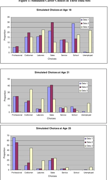
The occupational choice patterns in the three simulated data sets are summarized in Figure

1. The simulated choices in data sets 1 and 2 exhibit qualitatively similar choice-age „ †ˆ ‰les.

One noteworthy feature of the ‰rst two data sets is the large upward age trend in professional

employment, with Š‹ Œ of the workers in data set 1 working as professionals at age 25, and ‹ ‹Œ

of the workers in data set 2 working as professionals at age 25. Across all three simulated data

sets the proportion of people attending school declines sharply with age. This happens because the

declines with age. The simulated choices in data set 3 are quite Žerent from those in the rst

two data sets. Some of the largest dierences are that unemployment is quite common in the third

data set and professional employment is very rare compared to therst two data sets. In addition,

employment as craftsmen and laborers is much more common in the third data set compared to the

rst two data sets. Overall there is a more even choice distribution in the third data set compared

to therst two data sets.

‘’” •–s—˜ts™ Ass–ssš›œ t– ž–rŸ r¡a›c–  Ÿ t– ¢›t–r£ ˜atš › ¥–t ¦

Tables 1-4 present evidence on the performance of the interpolation method in each of the three

simulated data sets. Table 1 shows the proportion of simulated choices in the data generated using

interpolated value functions that match the choices found in the data generated without using

interpolation. Any dŽ erences between these simulated choices are the result of approximation

error in the interpolated value functions. For example, therst entry in therst column of Table 1

indicates that when Emax is simulated at§¨of the state space and interpolated at the remaining

© §¨ of the state space, 9©ª ©¨ of the choices in time period 1 in the simulated data match the

optimal choices when interpolation is not used. The percentage of correct choices is quite stable

across time periods, with an overall match rate of 99.«¨ across all time periods when©¬¨of the

state space is interpolated. Thenal entry in the rst column of Table 1 shows that the computer

program that interpolates Emax at 9§¨ of the state space runs 43 times faster than the program

that simulates Emax at all points in the state space. The amount of time it takes to solve the

dynamic programming problem is reduced from 6 hours to only 8 minutes when the value functions

are interpolated at 9§¨ of the state space.

­iven that the dynamic programing problem must be

solved repeatedly during the estimation of the parameters of a dynamic discrete choice model as a

greatly expands the scope of dynamic programming problems that are feasible to estimate.13

One striking feature of Table 1 is that the performance of the interpolating regression does not

appear to deteriorate as the number of state points used in the interpolating regression decreases.

The percentage of correct choices is constant at 99.6®when the value functions are interpolated at

¯ ° ®±¯ ¯ ®±or 99.² ®of the state space. Of course, the amount of time it takes to solve the dynamic

programming problem decreases as the level of interpolation increases because an increasing number

of relatively slow integral simulations are replaced by fast regression interpolations. Interpolating

the value functions at ¯ ¯ ® of the state space reduces computation time by a factor of 114, while

interpolating the value functions at¯ ¯ ³² ®of the state space reduces computation time by a factor

of 819.

The results shown in Table 1 indicate that the interpolating regression provides extremely

accurate predictions of Emaxeven when the value functions are interpolated at a very large fraction

of the state space. In some respects this is not surprising because in data set 1 the standard

deviations and e are relatively small, so one could do fairly well by interpolating Emax with

the extreme value solution [V_t+1(k)] without even estimating an interpolating regression: In other words, the co´µ cient estimates for the interpolating regression are quite close to !0t = 0

and !1t= 1 in many time periods for this set of parameter values. The error standard deviations

used to generate data set 1 are based on maximum likelihood estimates from the closely related

occupational choice model estimated in Sullivan (2006), so they should be considered reasonable

parameter values.14 These parameter estimates imply that there is more dispersion in random

1 3_{In most applications of dynamic programming models the computational burden of evaluating a likelihood}

func-tion or set of moment condifunc-tions during estimafunc-tion is insigni¶cant relative to the computational burden of solving

the dynamic programming problem. 1 4_{The major di}

·erences between the models presented in Sullivan (2006) and the one presented in this paper are:

1) For simplicity, this version of the model rules out within ¶rm occupational mobility, 2) The model in Sullivan

(2006) allows for person-speci¶c unobserved heterogeneity in occupation speci¶c ability ( ’s) and preferences ( ’s)

shocks to non-pecuniary utility than in random wage shocks or job match values.

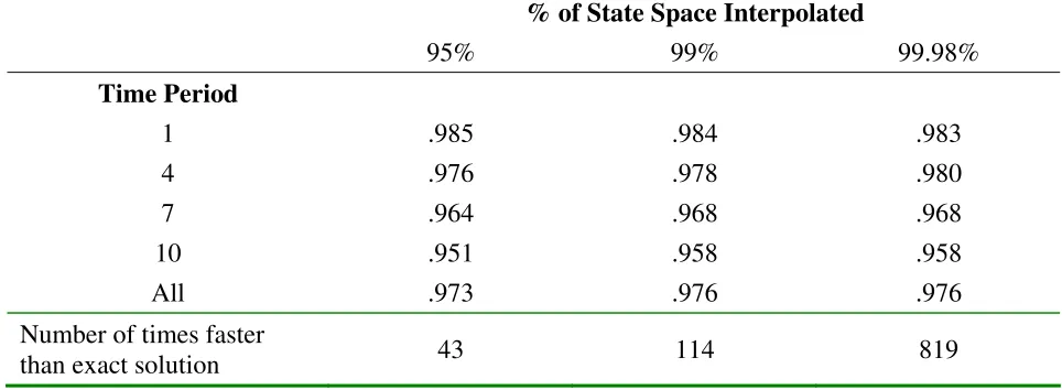
Table 2 examines whether the performance of the interpolating regression is robust to changes

in the standard deviations of the error terms in the model. Sp¹ º» ¼cally, data set 2 is generated using

parameter values that increase the importance of random wage shocks in determining career choices

relative to the¼rst data set. Most importantly, the error standard deviations are increased in such

a way that the extreme value solution for Emax( [V_t+1(k)]) used as the interpolating regressor is a poorer approximation of the actual value of Emax. As and eincrease, ( [Vt+1(k)]) becomes

a poor approximation of Emax because it does not capture the increasing option value of mobility

associated with large values of and e: Data set 2 reveals the extent to which the regression

parameters !0t and !1t are able to capture the departure of Emax from [Vt+1(k)] when the

importance of the non-extreme value error terms is large relative to the importance of the extreme

value error.

The results shown in Table 2 demonstrate that the interpolating regression performs extremely

well when the standard deviation of the normally distributed random wage shock is large relative

to the extreme value utility shock. The interpolating regression captures the additional option

value associated with an increase in the variance of the wage shocks through the constant in the

interpolating regression. The R-squared for the interpolating regression remained at approximately

:99in each time period. When the value functions are interpolated at 9½¾of the state space 9¿ ÀÁ¾

of the choices generated using interpolated value functions match the true choices. The match rate

declines slightly over time from 98.5¾ in time period 1 to 95.¾ in time period 10. This happens

because errors in simulated choices in one time period create errors in the state variables thatà Äect

the value of future choices. For example, suppose that interpolation error causes a choice in year 1

for a simulated person to be attending school instead of unemployment. Attending school ÃÄects

to choose to work in occupations where education is highly rewarded.

As in data set 1, the performance of the interpolating does not appear to deteriorate as the

value functions are interpolated at an increasingly large fraction of the state space. Interpolating

the value functions at 99.9ÆÇ of the state space allows the dynamic programming problem to be

solved 819 times faster than when the value functions are simulated across the entire state space,

but the interpolated value functions still lead to the optimal choiceÈÉ ÊËÇof the time. The overall

match rate of approximately ÈÉÇ in data set 2 is only slightly lower than the È ÈÇ match rate

found in data set 1. Overall, the performance of the interpolating regression using the second set of

parameter values is quite encouraging. The interpolating regression performs extremely well even

when the extreme value solution for Emaxis far from the true value of Emax.

Further information about the performance of the interpolating regression in data set 2 is shown

in Table 3, which presents the average percent absolute deviation of the interpolated value functions

from the actual value functions for the second data set. The entries in the table are computed using

the following formula

%Abs. Dev.= 100 ÌV(interpolated) V(exact)Ì ÌV(exact)Ì

;

averaged over all the value functions found in the simulated data. On average, the interpolated and

exact value functions Í ÎÏer by only .32Ç when the value functions are interpolated at ÈÈ ÊÈ ÆÇ of

the state space, so the interpolation method is extremely accurate. The magnitude of the percent

absolute deviation is virtually constant across all levels of interpolation, so these statistics are

not reported here for the ÈÐÇ and È ÈÇ interpolation levels. The excellent performance of the

interpolation method according to this metric is not surprising because the extremely close match

between the choices generated using the interpolated and exact value functions shown in Table 2 is

only possible if the interpolation method produces value functions that are extremely close to their

These results show that using the extreme value closed form solution for Emax( [V_t+1(k)]) in an interpolating regression performs extremely well even when the error standard deviations are set

at values such that [V_t+1(k)]is a poor approximation of Emax. The intuition behind this result is that the interpolating regression captures the departure of Emax from [V_t+1(k)]through the constant of the interpolating regression. As the option value of job search increases moving from

data set 1 to data set 2, the constant in the interpolating regression also increases.

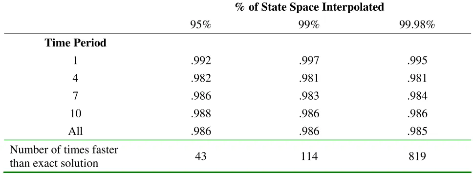
Table 4 presents evidence on the performance of the interpolation method in data set 3. The

third data set demonstrates substantiallyÔ ÕÖerent lifecycle choice patterns compared to the×rst two

data sets, as shown in Figure 1. The majorÔ Õ Öerence is that workers are more evenly distributed

across choices than in the ×rst two data sets. This implies that the value functions for the various

choices are closer to each other in magnitude in the third data set compared to the ×rst two data

sets, so there is more room for small interpolation errors to result in dÕ Öerences between the choices

generated using the interpolated and exact value functions. The results shown in Table 4 show that

the interpolation method performs quite well in the third data set, with approximately 98Øof the

interpolated choices matching the exact choices. As in the previous two data sets the performance

of the interpolation method is very stable as the fraction of the value functions that are interpolated

increases.

Ù ÚÛÜ

c

s

This paper presents a method of approximately solving dynamic discrete choice models that builds

on the simulation and interpolation method developed by àáâ ãe and Wolpin (1994). The key

assumption is that one of the error terms (unobserved state variables) in the model is distributed

extreme value. Other error terms may be freely incorporated to allow for various types of correlation

between the error terms associated with diÖerent choices in a given time period or between choices

remaining points in the state space using a new regression function based on the extreme value

closed form solution for the expected maxima of the value function.

One advantage of this approach is that when the standard deviations of the non-extreme value

error terms are small the interpolated value functions are guaranteed to be close to their actual

values since the interpolating regression function converges to the exact solution for Emax as the

standard deviations of the non-extreme value errors approach zero. On a more practical note, the

regression is based on a single regressor so it avoids the colinearity problems that can arise when

using interpolation methods that use individual expected value functions as regressors. Experience

shows that these problems are likely to arise across a wide range of parameter values in models

with large choice sets, especially when the structure of the model tends to produce choices that

have similar discounted expected values. In addition, the single regressor is dæ çned at each point

in the state space even if the choice set varies over the state space, so one does not need to estimate

multiple interpolating regressions corresponding to each feasible choice set.

The performance of the interpolating regression is evaluated using a dynamic model of career

choices that incorporates a large choice set and an error structure that incorporates correlation

across time due to job matching and correlation across choices within a given time period. The

performance of the interpolation method is evaluated using three sets of parameter values that

èéêer in the relative importance of the extreme value and non-extreme value errors and generate

èéêerent optimal choice sequences. Across all simulated data sets the interpolated value functions

generate choice sequences that are extremely close to the optimal choice sequences generated by

exact solution to the value functions. Evidence is also presented that the diêerences between the

interpolated and actual value functions are extremely small on average, on the order of a fraction

of a percentage point.

Overall, the evidence presented in this paper suggests that the interpolating regression based on

is a poor approximation to the actual value of Emax. This method appears to be well suited for use

in models with large choice sets and complicated error structures. The large decrease in the amount

of computation time associated with using interpolation to solve the dynamic programming problem

Figure 1: Simulated Career Choices in Three Data Sets

Simulated Choices at Age 18

0 5 10 15 20 25 30 35

Professional Craftsmen Laborers Sales Service School Unemployed

Choices P rop or ti o n Data 1 Data 2 Data 3

Simulated Choices at Age 21

0 10 20 30 40 50

Professional Craftsmen Laborers Sales Service School Unemployed

Choices P rop or ti o n Data 1 Data 2 Data 3

Simulated Choices at Age 25

0 10 20 30 40 50 60 70

Professional Craftsmen Laborers Sales Service School Unemployed

Table 1

Proportion Correct Choices – Data Set 1

% of State Space Interpolated

95%

99%

99.98%

Time Period

1 .999

.999

1.000

4

.998 .999 .998

7

.994 .995 .993

10

.993 .993 .992

All

.996 .996 .996

Number of times faster

than exact solution

43 114 819

Notes: Based on a simulated sample of 2,000 people. Emax is simulated using 100 draws of the errors and antithetic acceleration is used to reduce the variance of the simulated integrals. Entries represent the proportion of simulated choices generated using different levels of interpolation that match the simulated choices when the model is solved exactly (without interpolation).

Table 2

Proportion Correct Choices – Data Set 2

% of State Space Interpolated

95%

99%

99.98%

Time Period

1

.985 .984 .983

4

.976 .978 .980

7

.964 .968 .968

10

.951 .958 .958

All

.973 .976 .976

Number of times faster

than exact solution

43 114 819

Table 3

Percent Difference Between Simulated and Actual Value Functions – Data Set 2

% of State Space

Interpolated

99.98%

Time Period

1 .37%

4 .14%

7 .35%

10 .65%

All .32%

Notes: Based on a simulated sample of 2,000 people. Emax is simulated using 100 draws of the errors and antithetic acceleration is used to reduce the variance of the simulated integrals. Entries represent the percent absolute deviation of the simulated value functions from the actual value functions.

Table 4

Proportion Correct Choices – Data Set 3

% of State Space Interpolated

95%

99%

99.98%

Time Period

1

.992 .997 .995

4

.982 .981 .981

7

.986 .983 .984

10

.988 .986 .986

All

.986 .986 .985

Number of times faster

than exact solution

43 114 819

ëìíì

r

c

s

ïð ñ Aguirregabiria, Victor and Pedro Mira (2002).òSwapping the Nested Fixed Point Algorithm:

A Class of Estimators for Discrete Markov Decision Moó ôõö÷ ø Econometrica, v.ù0, no. 4.

ïúñ Aguirregabiria, Victor and Pedro Mira (2006).

òSequential Estimation of Dynamic Discrete

ûümôö÷ ø forthcoming in Econometrica.

ïý ñ Arcidiacono, Peter (2004). òAbility Sorting and the Returns to College Major÷ ø Journal of

Econometrics, v. 121: ý þý ÿýù 3÷

ï þñ Bellman, Richard(ð 3 ù ÷ òDynamic Pro ü ÷ ø Princeton University Press.

ï3 ñ Berkovec, James, and Steven Stern (1991).òJob Exit Behavior of Older Me÷nEconometrica,

v. 59, no. 1: 189-210.

ï[ ñ Berry, Steven (1992).òEstimation of a Model of Entry in the Airline Industry÷ øEconometrica,

v. 60, no. 4: 88 ÿ ðù ÷

ïù ñ Berry, Steven, James Levinsohn, and Ariel Pakes (1995).òAutomobile Prices in Market

Equi-librium.ø Econometrica, v. 63, no. 4: 841-890.

ï8 ñ Brien, Michael, Lee Lillard and Steven Stern (2006).òCohabitation, Marriage and Divorce in

a Model of MatchQüõ ty.øInternational Economic Review, v. þù, no. 2.

ï ñ Eckstein, Z i and Kô neth Wolpin (1989). òThe Spôe cation and Estimation of Discrete

Choice Dynamic Programming Models.ø Journal of Human Resources, v. 24: 562-598.

ïðñ ûôGeke, John (1988). òAntithetic Acceleration of Monte Carlo Integration in Bayesian

] H kman, James, and Burton Singer (1984). “A Method for Minimizing the Impact of

Dis-tributional Assumptions in Econometric Models for Duration Data.”Econometrica, v. 52:

2 2

2] H Joseph and Robert Miller (1993).“Conditional Choice Probabilities and the Estimation

of Dynamic Programming Mod Review of Economics and Statistics, v. 60: 4

] , Michael and neth Wolpin (1994).“The Solution and Estimation of Discrete Choice

Dynamic Programming Models by Simulation and Interpolation: Monte Carlo EvidencThe

Review of Economics and Statistics, v.6, no. 4: 64 ! 2

4] , Michael, and neth Wolpin " #.“The Career Decisions ofYoung Me”Journal

of Political Economy, v. 105 : 44 2

] Manski, Charles. “Nonparametric Estimation of Expectations in the Analysis of Discrete

Choice Under Uncertainty. In Nonparametric and Semiparametric Methods in Econometrics

and Statistics, edited by W. Barnett, J. Powell, and $ Tauchen. pp. 2 2 ! MIT Press,

Cambridge.

!] McFadden, Daniel (1981). “Econometric Models of Probabilistic Choice. In C. Manski and

D. McFadden (eds.)Structural Analysis of Discrete Data with Econometric Applications, pp.

2 2MIT Press, Cambridge.

] Miller, Robert A. (1984).“Job Matching and Occupational Choice ”Journal of Political

Econ-omy, v. 92: 1086-1120.

] Pakes, Ariel (1986).“Patents as Options: Some Estimates of the Value ofH ding European

Patent Stocks. Econometrica, v. 54, no. 4.

] Rust, John ( # “Optimal Replacement of $%& Bus Engines: An Empirical Model of

*+, - Rust, John (199 ./ 0 1Using Randomization to Break the Curse of Dimensionality.5

Economet-rica, v. 65, no. 3.

*+6- Rust, John (2005). 1Structural Estimation of Markov Decision Process7 :05 In Handbook of

Econometrics Vol. 4, edited by R. Engle and D. McFadden. North-;olland.

*+ +- Rust, John and Christopher Phelan<699./.1;=w Social Security and MedicareA >ect

Retire-ment Behavior in a World of Incomplete Mark7?:0@Econometrica, v. 65: .B6C BD60

*+ D- Stern, Steven (199./0 1Simulation Based Estimation.5 Journal of Economic Literature, v. 35,

no. 4.

*+E- Stinebrickner, Todd (2000).1Serially Correlated Variables in Dynamic Discrete Choice

Mod-7 F :05 Journal of Applied Econometrics, v. 15: 595-624.

*+I - Stinebrickner, Todd (2001).1A Dynamic Model of Teacher Labor Supply.5 Journal of Labor

Economics, v. 19, no. 1.

*+J- Sullivan, Paul (2006).1A Dynamic Analysis of Educational Attainment, Occupational Choices,

and Job Search.5 Working paper.

*+ .- Wolpin,L7 Mneth (1992).1The Determinants of Black-White Di>erences in Early Employment

Careers: Search, Lay=>s,NO i?s, and Endogenous WagePRowth.@Journal of Political Economy,

Appendix A: Utility Flow Equations

The remaining portion of the non-pecuniary utility function contains the non-pecuniary

em-ployment and non-emem-ployment utility ‡ows along with the schooling cost function. This utility

‡ow equation is speci…ed as

h(k; Sit) = hP5_q=1 q(Sit)1feqSkg

i

TU VW

+Cs(Sit)1fsSk; emp =Skg+C sw_(S

it)1fsSk; empSkg

+b(Sit)1fuSkg+C g_(S

it)1fgSkg:

The term in brackets contains the occupation and …rm speci…c non-pecuniary utility ‡ows. The

occupation spec X …c portion of this ‡ow, q(Sit), is a function of the state vector that is allowed

to vary over occupations. The second line of equation UV contains the schooling cost functions for

attending school while not employed (Cs(Sit)) and employed (Csw(Sit)). The …nal components of

the non-pecuniary utility ‡ow are the deterministic portions of the value of leisure enjoyed while

unemployed,b(Sit), and the cost function for earning a \ED, C g_(S

it).

The deterministic portion of the occupation sp^cX…c human capital wage function is

wq(Sit) = q1ageit+ q2age2it=100 + q3hsit+ q4colit+ q51[ageit _17]+ (28) q

61[ageit`18aageit_21] + q

7gedit

Let N Ft be a dummy variable indicating whether or not the individual is in his …rst year of

employment at a …rm after being employed at a dXberent …rm in the previous period. Let hdt

and cdt represent dummy variables that indicate receipt of a high school or college diploma. The

non-pecuniary utility‡ow equation for occupationq is

q(Sit) = q1ageit+ q2age2it=100 + q3(hsit+colit) + q6hdit (29)