Delay Analysis of ML MAC Algorithm For Wireless Sensor Networks

Delay Analysis of ML-MAC Algorithm For Wireless

Sensor Networks

Madhusmita Nandi

School of Electronics Engineering, KIIT University Bhubaneswar-751024, Odisha, India

ABSTRACT

The present work is to evaluate energy consumption in wireless sensor networks for multi-layer medium access control (ML-MAC) scheme where the delay times, i.e., packet transmission delay, maximum response time delay, clock-drift delay, sleep delay and queuing delay are considered. Sensor nodes in ML-MAC algorithm have very short listening time than sensor-MAC (S-MAC) which would minimize the energy. The number of collisions where two or more nodes try to send at the same time is reduced in ML-MAC. Simulation results of performance of ML-MAC compared with ML-MAC considering the delay time and S-MAC.

Keywords

Energy consumption, Medium access control (MAC), Wireless sensor networks.

1.

INTRODUCTION

Medium access control (MAC) is the part of the link layer in the OSI layer model and is central to the proper functioning of any communication system. Medium Access Control (MAC) algorithms are used to allow several users simultaneously to share a common medium of communication in order to gain maximum of channel utilization with minimum of interference and collisions. As most sensor nodes are battery operated and normally they cannot be recharged due to its deployment in harsh and remote environment[1]-[3]. Therefore, energy efficiency is a very critical issue to prolong the networks lifetime.

The contention based protocols use an active/sleep routine frame to save energy consumption. The frame length Tframe

comprises of the listen and the sleep time. It define the duty cycle as Tlisten/Tframe , Tlisten is the active (listen) time of a

cycle[4]. There are four major sources of energy waste: collision, overhearing, control packet overhead and idle listening. In IEEE 802.11, In the active/sleep cycle schemes, sensor nodes schedule-wise turn off their radio and go into sleep mode, which will reduce the idle listening excellently.

2.

SENSOR-MAC (S-MAC)

The basic concept of Sensor-MAC (S-MAC) algorithm is the synchronization management and sleep-listen schedules based on these synchronizations[1]. It uses cluster approach for communication, where some nodes close to each other form a virtual cluster. One of these nodes acting a leader called cluster head. Actually, the clusters are formed to set up a common sleep-listen schedule. It is possible that two neighboring nodes reside in two different virtual clusters, but they wake up for listening on the schedules of both clusters. This is the main drawback of S-MAC that the node has to follow two different schedules[5]. That results in more energy

consumption via extra listening and overhearing Figure 1 shows the listen and sleep schedule of S-MAC algorithm.

Figure 1: The schedule of listen and sleep in S-MAC

3.

OVERVEIW OF ML-MAC

ALGORITHM

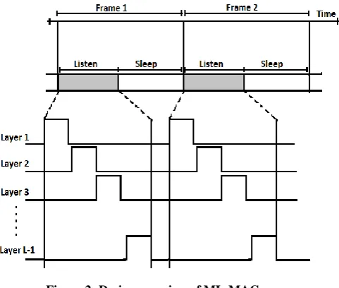
A multi-layer MAC (ML-MAC) algorithm is proposed as a technique to reduce node power consumption beyond that achieved by S-MAC. ML-MAC is a distributed contention-based MAC protocol where nodes discover their neighbors based on their radio signal level. It is also a self-organizing MAC protocol that does not need a central node to control the operation of the nodes. As Figure 2 shows, time in ML-MAC is divided into frames and each frame is divided into two schedule: listen and sleep. The active schedule is sub-divided into L non overlapping layers.

Figure 2: Design overview of ML-MAC

than the listen schedule of the frame in S-MAC. There are three main advantages of adopting multiple layers in ML-MAC: Reduced energy consumption, Low average traffic, Extended network lifetime.

Figure 3: Timing parameters of ML-MAC

4.

DESIGN OF ML-MAC ALGORITHM

To design a good MAC algorithm for wireless sensor network, there are so many reasons must be kept in mind. The most important is the energy efficiency. Steps for ML-MAC algorithm are[6]:

 The nodes are distributed into different layers using Uniform distributed function.

 Then traffic for each node in layers is generated according to a shifted Poisson's distribution function.

 Schedule is defined and it is dynamically changed according to the traffic in each layer of the frame conditions.

 If the sender and receiver nodes are in the same layer then no change has been made to scheduling otherwise the sender has to locate in the layer of the receiver. Hence has to wake in two layers in same active schedule.

 In this model first find which layer of the frame has the least amount of traffic. Then it changed the schedule of the receiver and sender node such that they will both wake in the layer of the frame with least traffic.

 Traffic is calculated using distribute matrix (nodes, layers, frames).Then nodes are ready to transmit packets in the layers.

 Sender does not have to wake twice in the same schedule. There will be less collision.

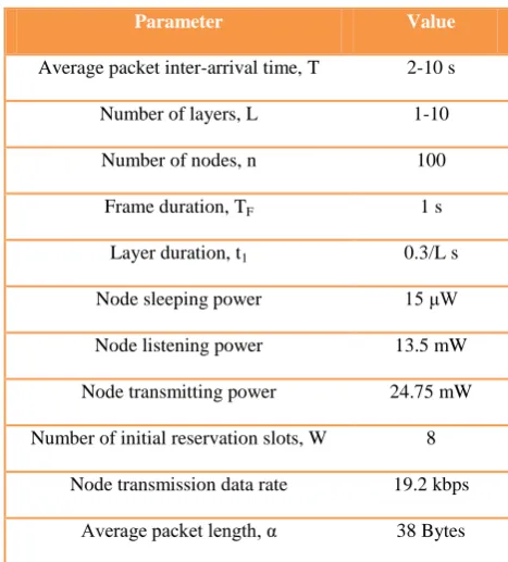
Design parameters are given in Table 1.

Table 1. Parameters are Assumed for Simulation

Parameter Value

Average packet inter-arrival time, T 2-10 s

Number of layers, L 1-10

Number of nodes, n 100

Frame duration, TF 1 s

Layer duration, t1 0.3/L s

Node sleeping power 15 μW

Node listening power 13.5 mW

Node transmitting power 24.75 mW

Number of initial reservation slots, W 8

Node transmission data rate 19.2 kbps

Average packet length, α 38 Bytes

The design parameters that need to be analyzed to study the achievement of ML-MAC. It has the following design specifications as shown in Figure 2 and Figure 3. Where,

L:Number of access layers

λ: Average packet rate per node

ρ:Average node power consumption

n:Total number of nodes in the network

g1:Guard time between slots.

TR: Maximum response time

TN: Network lifetime

τρ: Propagation delay

TF: Frame duration

τt: Packet transmission delay

τd: Clock drift delay

NF: Number of fames

t1: Layer duration

t2:Guard time between layers

The ML-MAC design procedure may be described as :

Step-1 : Calculating the frame duration TF

Maximum response time delay TR that is governed by the

time to respond the events, the frames duration TF is bounded

by:

(1)

For all layers, TF is bounded by total listening time:

Where t1 is the listening schedule per layer which is evaluated

in step 2:

Thus from equation (1) and (2), it is bounded as:

(3)

Step-2 : calculating the listening schedule per layer t1

The listening schedule of one layer t1 is governed by the

battery capacity C (mAh : mili ampere hour) and the average node power consumption ρ:

ρ (4)

Where V is the average output voltage of the battery. From equation (4), t1 is bounded as:

_ρ (5)

Also t1 is bounded by the time needed to send at least one

packet which is given by following equation:

τ τρ τ τρ (6)

Thus from equation (5) and (6), t1 is bounded as :

τρ τ τρ _ρ (7)

Step-3 : estimating the number of layers L

The number of layers determine by the average traffic generated per frame which is given by the below equation :

λ λ (8)

So, the total listen time should be greater than the time needed to send the entire packet generated by the nodes:

λ τ τρ τ τρ (9)

L is bounded as given below from equation (9)

λ τ τρ τ τρ

(10)

However, the guard time between layers t2 is governed by:

τρ τ (11)

Therefore, the upper limit in L is given in below:

(12)

Using equation (10) - (12), L should follow the below design bounds :

λ τ τρ τ τρ

(13)

To get the best behavior, it should determine the values of all timing parameters and the number of layers by using the delay limitations and buffer size in the node.

5.

TRAFFIC INTER-ARRIVAL TIME

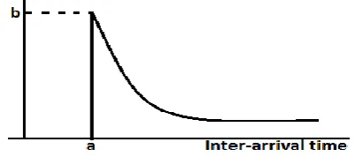
Poisson distribution used for the generation of traffic is described in the traffic inter-arrival model in Figure 4. It states that nodes statistically generate traffic that is based on an exponentially distributed inter-arrival time[6]. To test the algorithm's behavior for different arrival rates assume that the inter-arrival time between two successive packets be the random variable T, the probability density function (PDF) for the inter-arrival time of Poisson traffic follows the exponential distribution that can be written as [6]:

λ λ ₍₁₄₎

Where, λ is the average data rate, σ is maximum burst rate and α is the average packet length in bits. The inter-arrival time distribution is modified to get the shifted exponential distribution can be described as:

λ _{for (15)}

Where, a: Position parameter which represents the minimum time between adjacent packets, a > 0 and b: The shape parameter that describe how fast the exponential function decays with time. The values of a and b for a source with parameters λ, σ and α can be evaluated as:

α_σ (16)

_{α σ}σλ_λ (17)

λ (18)

σ (19)

is a constant value between 1 and T-1, but for simulation it has taken 1. The average inter-arrival time T of the packets in this simulation was taken from 2-10 s and the average packet length α was assumed to be fixed with only 38 bytes as most of the wireless networks have a small packet size.

Figure 4: Biased exponential distributed with the two parameters ‘a’ and ‘b’

Delays in ML-MAC: There are so many MAC delays are present in wireless communication[7] , i.e.,

Maximum response time delay: The response time of a task is defined as the time elapsed between the dispatch (time when task is ready to execute) to the time when it finishes its job.

Packet Transmission Delay: Transmission delay is

transmission delay in seconds, N is the number of bits, R is the rate of transmission (bits per second).

Propagation delay: Propagation delay is determined by the distance between the sending and receiving nodes and two thirds the speed of light. Propagation delay=d/s, where d=Length of physical link, s=Propagation speed in medium.

Carrier sense delay: when the sender performs carrier sense, the carrier sense delay is produced. Its value is found by the contention window size.

Processing delay: The processing delay mainly depends on the computing power of the node and the efficiency of the network data processing algorithms.

Queuing delay: Queuing delay depends on the traffic load and congestion level of router. In the heavy traffic, queuing delay becomes a dominant factor.

6.

RESULTS OF ML-MAC

Parameters of Table-1 are used in simulation and time is divided into frames of 1s duration and the simulation time is of 200s. So the number of frames is 200 and number of nodes is 100. The duty cycle is 33% which makes the duration of the listen schedule 300ms for the S-MAC. However, for the ML-MAC with L layers, the listen schedule is 300 ms. The size of data packet is fixed with 38 bytes which takes only 20ms to send in a typical radio channel. The traffic is analyzed by advancing the time index and checking for packets until the end of simulation. In this simulation, the time index is set to be frame duration/1000, i.e., frames are divided into 1000 slots.

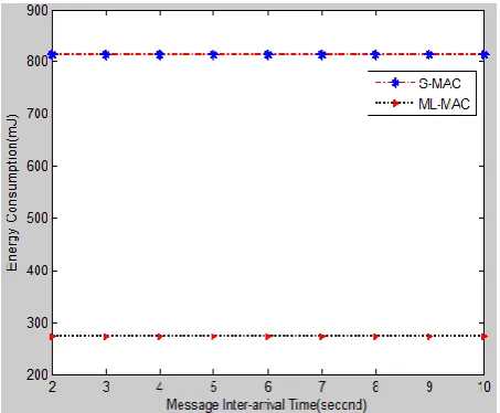
The total energy consumed by each node over the entire simulation time is determined by calculating the time each node spends in the three modes, i.e., listen, transmit and sleep. Then, the total time nodes spend in each mode is multiplied by the amount of power consumed in that mode to get the total energy consumed by the node.

Figure 5: Total energy consumption per node for S-MAC and ML-MAC with L=3; for the coherent case

If all the traffic emanating from node is destined to other nodes in the same access layer, i.e., the transmitter and receiver are in the same layer, then nodes do not have to wake up at different layers. This case is called the coherent traffic.

Figure 5 shows the energy consumption in coherent case. This shows how ML-MAC saves energy in compare to S-MAC. When the traffic is light, ML-MAC consumes 67% less energy than S-MAC.

Figure 6 Total energy consumption per node for ML-MAC taking delay and without delay with L=3; for the

non-coherent case

In Figure 6, here is considering 4 delays i.e. transmission delay, queuing delay, maximum response delay, clock drift delay. The clock drift delay is taken as 0.5 ms [6].Without taking delay the energy consumption is less. But taking the above 4 delays, the energy consumption of ML-MAC is large. When the message inter-arrival time is less than about 5s, ML-MAC with delay consumes 41% less energy than S-MAC and when the message inter-arrival time is greater than about 5s, it consumes 62% less than S-MAC. When the traffic is heavy, i.e., the message inter-arrival time is less than about 5s, ML-MAC without delay consumes 55% less energy than S-MAC and when the traffic is light, i.e., the message inter-arrival time is greater than about 5s, ML-MAC without delay consumes 65% less than S-MAC.

Figure 7: Energy consumption per node for ML-MAC in the non-coherent case, traffic is fixed:λ=0.2 packets/s

to L=5. However, after five layers, energy saving is not significant as most of the packets are destined to others layers and the nodes spend more time waking up at different schedules. Also, this increases the number of control packets that consumes more energy. It is the total energy consumed in a node for the whole simulation time, as the number of layers L is increased from 1 to 10 layers using non-coherent traffic.

Sensor-MAC(S-MAC) [1] consists of three major components: scheduled listen and sleep, collision and overhearing avoidance and message passing. The scheduled listen and sleep states that if in each second a node sleeps for half second and listens for the other half, its duty cycle is reduced to 50%. so It can achieve close to 50% energy savings. An extra delay in S-MAC is caused by nodes scheduled sleeping. When a sender gets a packet to send, it must wait until the receiver wakes up. It is called as sleep delay as it is caused by the sleep of the receiver. A complete cycle of the listen and sleep is a frame. Assume a packet arrives at the source with equal probability in time within a frame. So the average sleep delay on the sender is

where (20)

The relative energy savings in S-MAC is

(21)

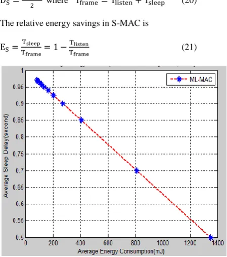
Figure 8: Average energy consumption verses average sleep delay per node for ML-MAC

Figure 8 shows the percentage of time when each node is in the sleep mode for S-MAC in this simulation is fixed at 70% because it has a fixed duty cycle. [6] However, for the same duty cycle, nodes in ML-MAC sleep about 90% of the time and vary depending on the traffic type for the non-coherent case.

Figure 9 Average delay for all packets sent for ML-MAC in the non-coherent case, traffic is fixed:λ=0.2packets/s

Figure 9 shows the effect of adding more layers on delay for the non-coherent traffic. If the number of layers is less than three, then delay would increase rapidly. But, when more layers are added, then packets will not encounter more delay as they are usually buffered for the next or third frame cycle.

Figure 10 Average delays for all packets sent for the protocol, ML-MAC with L=3; in the non-coherent case

message inter-arrival time is greater than about 5s, it consumes 18% less delay than ML-MAC taking 4 delays, i.e., queuing delay, transmission delay, clock-drift delay and maximum response delay consideration.

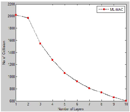
Figure 11: Number of collisions for ML-MAC in the non-coherent case, λ=0.2packets/s

Figure 11 shows how the number of collisions declines dramatically by adding more layers for ML-MAC using the non-coherent and fixing the traffic at 0.2 packet/s. However, after about 6 layers, it stops decreasing significantly because packet requests per layer spread out enough such that the chance of collision is reduced for this type of traffic. The high number of collision in the last result is due to the traffic type generated for the simulation. The values of two traffic parameters λ and σ are 0.2 and 0.25 packets/s, respectively. Because λ and σ are close to each other, then all 100 nodes generate packets that have around the same arrival times. As a result the number of collision is high.

Figure 12: Probability of collisions for ML-MAC in the non-coherent case, traffic is fixed:λ=0.2packets/s

Figure 12 shows, when traffic is heavy, more packets are generated. When the message inter-arrival time is above 5s then traffic is light, less packets are generated. The formula of probability of collisions is given below:

(22)

7.

CONCLUSION

ML-MAC is an energy-efficient MAC algorithm in WSNs. In this algorithm, nodes are distributed in layers in order to minimize the idle listening time. The simulation and results shows the energy consumption of ML-MAC without delay comparing with S-MAC and ML-MAC with delay. Comparison of energy consumption using delays with communication controlled MAC algorithm for WSNs is one of the future works. Further research work on this topic may be extension of the MAC algorithm method for energy consumption for varying traffic load. With the specified parameters assumption, the results of ML-MAC algorithm with delay are showing ML-MAC with delay outperforms S-MAC and ML-S-MAC without delay in conserving energy by having an extremely low duty cycle and minimizing the probability of collisions.

8.

REFERENCES

[1] Ye, W., Heidemann, J., Estrin, D. An energy-efficient MAC protocol for wireless sensor networks. IEEE INFOCOM 2002, Vol.3, 1567-1576.

[2] Ye, W., Heidemann, J., Estrin, D. Medium access control with coordinated adaptive sleeping for wireless sensor networks. IEEE/ACM Transactions on Networking, 2004, Vol. 12, No.3, 493-506.

[3] Koutsakis, P. 2006. On increasing energy conservation for wireless sensor networks. Technical University of Crete. ICWMC-06 (July 2006), 4-14.

[4] Singh, S., Raghavendra, C. S. 1998. PAMAS-power aware multi-access protocol with signalling for ad-hoc networks. ACM SIGCOMM Computer Communication Review (July 1998). 5-26.

[5] Jurdak, R., Lopes, C. V., Baldi, P. 2004. A survey, classification and comparative analysis of medium access control protocols for ad hoc networks. IEEE Communications Surveys & Tutorials, 2-16.

[6] Jha, M. K., Pandey, A. K., Pal, D., and Mohan, A. 2011. An energy efficient multi-layer MAC (ML-MAC) protocol for wireless sensor networks. International Journal of Electronics and Communications (AEU) 65, 209-216.