Comparing Action as Input and Action as Output in a Reinforcement Learning Task

Comparing Action as Input and Action as Output in a

Reinforcement Learning Task

Evans Miriti

School of Computing and Informatics University of Nairobi

Peter Waiganjo

School of Computing and Informatics University of Nairobi

Andrew Mwaura

School of Computing and Informatics University of Nairobi

ABSTRACT

Generalization techniques are useful for enabling an agent to be able to approximate the value of states it has not encountered so far in reinforcement learning. They are also useful as memory use minimization mechanisms in situations where the state space is too large such that is infeasible to represent every state in the state space in the computer memory. Artificial Neural Networks are one generalization technique that is usually employed. Various network structures have been proposed in literature. In this study, two of the structures that have been proposed were implemented in a robot navigation task and their performance compared. The results indicate that having a network structure where there is an output node for each of the possible actions, is superior to the structure in which the selected action is fed as an input to the network and its value output by the single network output node.

General Terms

Reinforcement Learning, Artificial Neural Networks, obstacle avoidance.

1.

INTRODUCTION

A Reinforcement Learning (RL) agent learns by interacting with the environment and based on the outcome of the interaction, learns to select the actions that lead to the most desirable outcomes. Thus by sensing and acting in its environment an RL agent can learn to choose optimal actions to achieve its goals. Every time an agent performs an action in the environment, it receives a reward or a penalty to indicate the desirability of the resulting state. Since the agent does not know beforehand which are the optimal actions, it must learn via a trial and error process (Kaelbling et al., 1996). For example a game playing agent may receive a positive reward for a winning state, a negative reward for a losing state, and a zero reward for all other states. The task of the agent is to learn from this indirect delayed reward to choose sequences of actions that produce the greatest cumulative reward (Mitchel, 1997).

The outcome of the agent learning is a control policy (). The policy can be defined as a function : SA that outputs an appropriate action a, given a state s, where S is the set of states and A is the set of actions (Mitchel, 1997).

For tasks with small state spaces and action sets, the value of each state or state-action pair can be stored in a table with one entry for each state or state-action pair (Sutton & Barto, 1998). As the number of states/ state-action pairs increases, several problems will arise

i. The table will become too large hence there may not be enough memory to store it, or too much memory will be required.

ii. During exploration, some of the states/ state-action pairs will not be experienced hence their values will not be set or too much time will be required to perform enough exploration to fill all the table entries with reasonable value estimates. Function approximation is the technique used to deal with this problem. Function approximators are used to generalize from previously experienced states to ones that have never been seen (Sutton & Barto, 1998). Artificial neural networks using a modified form of the back-propagation training algorithm are one technique that has been used for function approximation (Tesauro, 1995). Several alternative setups are proposed in (Mitchel, 1997). One option is to have a network with the state and action being inputs, and the value function being the output. A second option is to have a separate network for each action where the state as an input is fed to each of the networks and using the -greedy strategy, the action associated with the network that produces the greatest output value would be selected. A third option is to have one network with an output for each action. If a neural network is used as the function approximator, the TDBackpropagation algorithm can be used for training (McClelland, 2013), (Sutton S Richard , 1998). (Mitchel, 1997) Notes that using one network for each of the outputs has been found to be more successful.

In his study, the performance of two of the network structures described above were compared. First, the structure where we have the action as an input and second, the structure where we have the action as an output. These were compared in a robot control task.

2.

ACTION AS INPUT ARTIFICIAL

NEURAL NETWORK

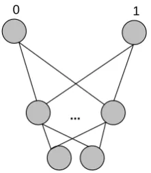
0

1

2

3

...

...

Figure 1: An Action as input Multilayer Artificial Neural Network for a two variable state, and 2 possible actions.

In figure 1, if we have actions A and B, input node 2 can be associated with action A and input node 3 with action B. To get the value for action A in state s, the state variable values are input in node 0 and 1, and node 2 is set to 1 (action A selected) while node 3 is set to zero (action B not selected). To get the value of action B in the same state, the inputs for node 0 and 1 remain the same, while node 2 is set to zero (action A not selected) and node 3 to 1 (action B selected). Consequently, the action value is calculated twice (or as many times as there are actions).

3.

ACTION AS OUTPUT NETWORK

STRUCTURE

In this structure, the output is the state-action value of each action, but the network has several outputs, one for each of the actions. After computing the values of the outputs, the action corresponding to the output node with the greatest value is the currently best action.

0 1

...

Figure 2: An Action as out Multilayer Artificial Neural Network for a two variable state, and 2 possible actions.

4.

EXPERIMENTAL TASK

Robot obstacle avoidance deals with the local observable aspect (within the robots perception horizon), where the robot may detect some unknown obstacles (real-time obstacles) on its path to an observable point (goal) (Kane Usher, 2006). This problem can be simplified so that there are no obstacles in the environment, and the task of the control agent is to move the robot towards the goal once the goal is sighted. A two wheel differential drive robot enables the setting of the

are set to the same speed at the same speed, then the robot moves in a straight line.

The robot is rewarded for reaching the goal and so it needs to be able to select the action(s) which lead it to the goal. Since there are no obstacles in the environment, once the goal is sighted, the best policy is to choose the action that generates a straight path to the goal if this is one of the available actions. Rewarding the robot only when it reaches the goal results in a sparse reward function which makes it very hard for the robot to learn the desired steering function because it hardly ever reaches the goal. Note however that it is very easy to solve this problem using structured programming. The robot is just programmed to turn until the goal is sighted. Once the goal is sighted, the robot selects the action which results in a straight line movement towards the goal. The objective of this work was to determine the performance of the two different network structures in learning to perform this task.

5.

Experimental Setup

The reward function was set up such that the agent got a reward of 1 when the goal was reached and 0 otherwise. Since it is possible for the robot to go on forever without reaching the goal, the number of steps (corresponding to actions) per episode is bounded (Sherstov & Stone, 2005). If the agent executes the maximum number of actions without reaching the goal, then the episode is terminated and a reward of -1 is awarded. Various values for the discount rate can be tried but since the episodes have a finite number of steps, then a discount rate of 1 was used.

To make the learning problem easier, the number of actions was reduced to 2. An action for turning left, and an action for moving straight ahead. These correspond to the following values for the left and right wheel powers (0, 0.1), (0.1, 0.1). These are low speeds but they do serve to illustrate the problem.

To ensure that the robot has a higher chance of reaching the goal, the distance to the goal was reduced so that it was as short as feasibly possible. This was done after the observation that the further the robot is from the goal, the lower the chance of its ever accidentally reaching the goal (which is necessary for initial learning). This is a form of learning from easy missions (Asada et al., 1994), (Taylor & Stone, 2005). The robot was also set so that the initial direction at the beginning of an episode was random relative to the goal. This meant that sometimes, in the initial position, the robot would be facing the goal, while at other times it would be facing away from the goal.

Each training trial lasted was limited to 100 episodes. TDBackpropagation (McClelland, 2013) as used as the training algorithm. The discount rate was set to 1 and the trace-decay parameter was set to 0.8. 5 hidden nodes were used for the action as input structure and 3 hidden nodes for the network as output structure. The learning rate was set to 0.1. The -greedy action selection strategy was used with the  initially set to 0.3 and being reduce by 0.01 after every 10 episodes.

A simulation environment Microsoft Robotics Developer Studio version 4(RDS) was used to create the above setup. The robot used was the P3DXMotorBase which is a simulated

version of Adept MobileRobots’ Pioneer P3-DX mobile robot (Microsoft, 2011).

6.

RESULTS

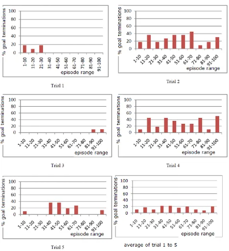
Figure 3: The percentage number of times the goal was reached in five trials using the action as input network structure.

In each trial in figure 3, the first bar represents the percentage number of times the goal was reached in the first 10 episodes, the second bar the percentage number of times the goal was

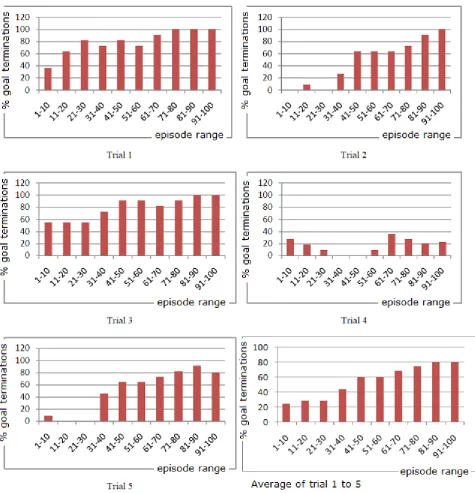
Figure 4: The percentage number of times the goal was reached in five trials using the action as output network structure

7.

DISCUSSION

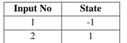
The performance in the first set of trials indicate that the action as input network structure is not a good choice for this learning task. The table below shows the expected inputs

Table 1: Inputs to the action as Input ANN.

Input No State A B

1 -1 1 0

2 -1 0 1

Table 1 represents the inputs for the action as Input ANN. Columns A and B represent the action. When A is on, the network is calculating the value of action A for the current state, and When B is on, the network is calculating the value if action B for the current state. We have only one state variable. Action A makes the robot move in a straight line, while B makes the robot turn

When the goal is visible, the network output values for input 3 and 4 are compared. If the output for 3 is greater, then action A (move straight) is executed. If the output for 4 is greater, then action B (turn) is executed. For the right behaviour, the output for 3 should always be greater so that the robot can move straight towards the goal.

In all the training episodes for the action as input network, outputs corresponding to 2 and 3 did not become greater at the same time hence showing that the network was not learning the right behaviour.

At any one time, either 1 and 3 were always greater or 2 and 4. This implies that the same action as the greater value both when the goal is visible, and when the goal is not visible. The agent either learns to move straight if the goal is visible or not, or to turn if the goal is visible or not. For our future experiments, this network structure was thus abandoned.

Table 2: Inputs to the action as output ANN.

Input No State

1 -1

2 1

When the actions correspond to output nodes, then we have 2 output nodes where the first node (A), corresponds to the action move straight, and the second output node (B) corresponds to the turn action. Input number 1 corresponds to the state when the goal is invisible, and input number 2 corresponds to the state when the goal is visible.

For the right behaviour, when the input is 1 (invisible), the output for the second node (turn) should be greater, and when the input is state 2 (visible), the output for the first node (straight) should be greater. We found that the network learns this behaviour in most of the trials as shown in figure 4. Trial 4 in figure 4 looks like an exceptions, but in the limit, the network does eventually learn. Hence for any future experiments, we choose to use the action as output structure. In the action as input setup, the robot does reach the goal sometimes, but this can be attributed to the stochastic nature of the policy, hence the robot is able to reach the goal by luck sometimes.

8.

CONCLUSION

This study provide evidence that the action as output structure is superior to the action as input structure for a neural network. This will be useful for persons wishing to use ANNs as the function approximation technique in reinforcement learning.

9.

FURTHER WORK

The number of state variables in this work is limited to just one. Further experiments can be done with more state variables.

An additional network structure involves having a separate network for each action. We intend to try this out in our future experiments.

10.

REFERENCES

[1] Asada, M., Noda, S., Tawaratsumida, S. & Hosoda, K., 1994. Vision-Based Behavior Acquisition for a Shooting robot by Using a Reinforcement Learning. In IAPR/IEEE Workshop on Visual Behaviours., 1994.

[2] Kaelbling, L.P., Littman, M.L. & Moore, A.W., 1996. Reinforcement Learning: A Survey. Journal of Artificial Intelligence,4 , pp.237-285. Available Through: CiteSeer [Accessed 7 August 2013].

[3] McClelland, J.L., 2013. Explorations in Parallel and Distributed Processing: A Handbook of Models, Programs and Exercises.

[4] Microsoft, 2011. Robotics Developer Studio: Getting Started.

[5] Mitchel, T., 1997. Machine Learning. Singapore: McGraw-Hill.

[6] Sherstov, A.A. & Stone, P., 2005. Improving Action Selection in MDPs via Knowledge Transfer. In 20th National Conference on Artificial Intelligence. Pittsburgh, USA, 2005. last accessed online on: http://www.cs.utexas.edu/~pstone/Papers/bib2html/b2hd-AAAI05-actions.html.

[7] Sutton S Richard, 1998. Implementation Details of the TD(gamma) Procedure for the Case of Vector Predictions and Backpropagation.

[8] Sutton, S.R. & Barto, G.A., 1998. Reinforcement Learning: An Introduction. London: MIT Press.

[9] Taylor, M.E. & Stone, P., July 2005. Behavior Transfer for Value-Function-Based Reinforcement Learning. In Fourth International Joint Conference on Autonomous Agents and Multiagent Systems. Utrecht, The Netherlands, July 2005.

[10]Tesauro, G., 1995. Temporal Difference Learning and TD-Gammon. Communications of the ACM, 38(3). [11]Usher, K., 2006. Obstacle avoidance for a