Numerical Solution of Fifth Order Boundary Value
Problems by Galerkin Method with Quartic B-splines
K.N.S.Kasi Viswanadham
Department of Mathematics National Institute of TechnologyWarangal – 506 004 (INDIA)
Sreenivasulu Ballem
Department of Mathematics National Institute of TechnologyWarangal – 506 004 (INDIA)
ABSTRACT
A finite element method involving Galerkin method with quartic B-splines as basis functions has been developed to solve a general fifth order boundary value problem. The basis functions are redefined into a new set of basis functions which vanish on the boundary where Dirichlet type of boundary conditions and Neumann boundary conditions are prescribed. The proposed method was applied to solve several examples of fifth order linear and nonlinear boundary value problems. The solution of a non-linear boundary value problem has been obtained as the limit of a sequence of solution of linear boundary value problems generated by quasilinearization technique. The obtained numerical results are compared with the exact solutions available in the literature.
Keywords
Galerkin method; Quartic B-spline; Basis function; Fifth order boundary value problem; Absolute error.
1.
INTRODUCTION
In this paper, we consider a general fifth order linear boundary value problem given by
)
1
(
),
(
)
(
)
(
)
(
)
(
)
(
)
(
)
(
)
(
)
(
)
(
)
(
)
(
5 4
3 2
) 4 ( 1 ) 5 ( 0
d
x
c
x
b
x
y
x
a
x
y
x
a
x
y
x
a
x
y
x
a
x
y
x
a
x
y
x
a
subject to boundary conditions
2 1
1 0
0
,
(
)
,
(
)
,
(
)
,
(
)
)
(
c
A
y
d
C
y
c
A
y
d
C
y
c
A
y
(2)where A0, C0, A1, C1 and A2 are finite real constants and a0(x),
a1(x), a2(x), a3(x), a4(x), a5(x) and b(x) are all continuous
functions defined on the interval [c, d].
Generally, this type of fifth order boundary value problem arises in the mathematical modeling of viscoelastic fluids and other branches of mathematics, physical and engineering sciences [1, 2]. The existence and uniqueness of the solution for these problems have been discussed in Agarwal [3]. Solving such boundary value problems analytically is possible only in very rare cases. So, many numerical methods have been developed overs the years to approximate the solution for these type of boundary value problems. Some of the already established methods are Finite difference method, Homotopy analysis method, Optimal homotopy analysis method, Spectral shifted jacobi tau and Collocation method, Variation of parameters method, Variational iteration method, Homotopy perturbed method, Residual correction method, Local polynomial regression method, Decomposition method, Sinc Galerkin method, Adomain decomposition method etc.
In the following, the attention is paid to the spline functions technique which has been developed to solve these type of boundary value problems. Davies A.R et al. [1, 2] were developed two numerical techniques namely, Spectral Galerkin and Spectral Collocation methods to solve fifth order boundary value problems, Fyfe [4] used spline functions to solve fifth order boundary value problems, who used quintic polynomial spline functions to develop consistency relation connecting the values of solution with fifth order derivative at the respective nodal points, Siddiqi et al. [5] presented the solution of special case of fifth order boundary value problems by using quartic spline functions, Siddiqi and Gazala [6,7] presented the solution of special case of fifth order boundary value problems by using sextic polynomial and non-polynomial spline functions respectively, Rashidinia et al. [8, 9] developed the solution of fifth order boundary value problems with mixed boundary conditions and boundary conditions of the type (2) by using sextic B-spline Collocation method and non-polynomial sextic spline off step method respectively, Caglar et al. [10] developed the solution of special type of fifth order boundary value problems by Collocation method with sixth degree B-splines, Siraj ul-Islam and Muhammad Azam Khan [11] presented the solution of special case of fifth order boundary value problems by using sextic spline functions, Feng-Gong Lang and Xiao-Ping Xu [12, 13] developed the solution of special case of fifth order boundary value problems by using cubic and quartic B-spline Collocation methods respectively, Lamnii et al. [14] applied sextic B-spline Collocation method to solve special case of fifth order boundary value problems, Kasi Viswanadham and Murali krishna [15] developed the quintic B-spline Galerkin method to solve special case of fifth order boundary value problems, Kasi Viswanadham and Showri raju [16, 17] developed the cubic and quartic B-spline Collocation methods to solve fifth order boundary value problems, Kasi Viswanadham et al. [18] developed the sextic B-spline Collocation method to solve special case of fifth order boundary value problems. So far, fifth order boundary value problems have not been solved by using Galerkin method with quartic B-splines. This motivated us to solve a general fifth order boundary value problem by Galerkin method with quartic B-splines.
been presented and followed by the proposed method with subject to boundary conditions. In Section 4, the procedure to solve the nodal parameters has been presented. In section 5, the proposed method is tested on several linear and nonlinear boundary value problems. The solution to a nonlinear problem has been obtained as the limit of a sequence of solution of linear problems generated by the quasilinearization technique [19]. Finally, in the last section, the conclusions are presented.
2.
JUSTIFICATION FOR USING
GALERKIN METHOD
For the few decades, the finite element method has become very powerful, useful tool to solve the boundary value problems in the complex dynamical systems. In finite element method (FEM) the approximate solution can be written as a linear combination of basis functions which constitute a basis for the approximation space under consideration. FEM involves variational methods like Rayleigh Ritz, Galerkin, Least Squares and Collocation etc.
In Galerkin method, the residual of approximation is made orthogonal to the basis functions. When one uses Galerkin method, a weak form of approximation solution for a given differential equation exists and is unique under appropriate conditions [20, 21] irrespective of properties of a given differential operator. Further, a weak solution also tends to a classical solution of given differential equation, provided sufficient attention is given to boundary conditions [22]. That means the basis functions should vanish on the boundary where the Dirichlet type of boundary conditions are prescribed. Hence in this paper the use of Galerkin method with quartic B-splines as basis functions has been employed to approximate the solution of fifth order boundary value problems.
3.
DESCRIPTION OF THE METHOD
Definition of quartic B-spline:
The quartic B-splines are defined in [23-25]. The existence of quartic spline interpolate s(x) to a function in a closed interval [c, d] for spaced knots (need not be evenly spaced) of a
partition
c
x
0
x
1
...
x
n1
x
n
d
is established by constructing it. The construction of s(x) is done with the help of the quartic B-splines. Introduce eight additional knots x-4, x-3, x-2, x-1, xn+1, xn+2, xn+3 and xn+4 in sucha way that
x-4<x-3<x-2<x-1<x0 and xn<xn+1<xn+2<xn+3 <xn+4.
Now the quartic B-splines
B
i(
x
)'
s
are defined by
otherwise
x
x
x
x
x
x
x
B
r i ir i
i r i
,
0
]
,
[
,
)
(
)
(
)
(
2 34 3
2
where
x x if
x x if x x x
x
r r r
r
, 0
, ) ( ) (
4 4
and
3(
)
)
(
i
r
x
x
x
where {B-2(x), B-1(x), B0(x), B1(x),…,Bn-1(x), Bn(x), Bn+1(x)}
forms a basis for the space
S
4(
)
of quartic polynomial splines. Schoenberg [25] has proved that quartic B-splines are the unique nonzero splines of smallest compact support with the knots atx-4<x-3<x-2<x-1<x0<x1<…<xn-1<xn<xn+1<xn+2<xn+3<xn+4.
To solve the boundary value problem (1) and (2) by the Galerkin method with quartic B-splines as basis functions, the approximation for y(x) can be defined as
1 2)
(
)
(
n
j
j j
B
x
x
y
(3)where
j'
s
are the nodal parameters to be determined. In Galerkin method the basis functions should vanish on the boundary where the Dirichlet type of boundary conditions are specified. In the set of quartic B-splines {B-2(x), B-1(x), B0(x),…, Bn-1(x), Bn(x), Bn+1(x)} the basis functions B-2(x), B-1(x),
B0(x), B1(x), Bn-2(x), Bn-1(x), Bn(x) and Bn+1(x) do not vanish at
one of the boundary points. So, there is a necessity of redefining the basis functions into a new set of basis functions which vanish on the boundary where the Dirichlet type of boundary conditions are specified. Since, the fifth order boundary value problem is going to be approximated by quartic B-spline polynomial, the basis functions are to be redefined into a new set of basis functions which vanish on the boundary where the Dirichlet and Neumann type of boundary conditions are prescribed. The procedure for redefining the basis functions is as follows.
Using the definition of quartic B-splines and the Dirichlet boundary conditions of (2), the approximate solution at the
boundary points can be written as
)
(
)
(
)
(
)
(
2 2 0 1 1 0 0 0 00
y
c
B
x
B
x
B
x
A
1B
1(
x
0)
(4))
(
)
(
)
(
)
(
2 2 1 10
y
d
nB
nx
n nB
nx
n nB
nx
nC
n1B
n1(
x
n)
(5)
Eliminating
2 and
n1from the equations (3), (4) and (5), the approximation for y(x) can be written as
nj
j j
P
x
x
w
x
y
1
1
(
)
(
)
)
(
(6)where
)
(
)
(
)
(
)
(
)
(
11 0 2
0 2
0
1
B
x
x
B
C
x
B
x
B
A
x
w
nn n
and
.
,
1
,
2
,
)
(
)
(
)
(
)
(
)
8
(
3
,...,
3
,
2
,
)
(
1
,
0
,
1
,
)
(
)
(
)
(
)
(
)
(
1 1 2 0 2 0n
n
n
j
x
B
x
B
x
B
x
B
n
j
x
B
j
x
B
x
B
x
B
x
B
x
P
n n n n j j j j j jUsing the Neumann boundary conditions of (2) to the approximate solution y(x) in (6), we get
)
(
)
(
)
(
)
(
1 0 1 1 0 0 0 01
y
c
w
x
P
x
P
x
A
1P
1
(
x
0)
(9)
)
(
)
(
)
(
)
(
1 2 2 1 11
y
d
w
x
n nP
nx
n nP
nx
nC
nP
n
(
x
n)
(10)
Eliminating
1 and
n from the equations (6), (9) and (10), we get approximation for y(x) as
1 0)
(
~
)
(
)
(
n j j jB
x
x
w
x
y
(11)where
)
(
)
(
)
(
)
(
)
(
)
(
)
(
)
(
1 11 0 1 0 1 1
1
P
x
x
P
x
w
C
x
P
x
P
x
w
A
x
w
x
w
n n n n
and (12)
.
1
,
2
,
)
(
)
(
)
(
)
(
3
,...,
3
,
2
,
)
(
1
,
0
,
)
(
)
(
)
(
)
(
)
(
~
1 0 1 0n
n
j
x
P
x
P
x
P
x
P
n
j
x
P
j
x
P
x
P
x
P
x
P
x
B
n n n n j j j j j j (13)Now the new set of basis functions for the approximation y(x)
is
{
B
~
j(
x
),
j
0
,
1
,
2
,...,
n
1
}
. Applying the Galerkin method to (1) with new set of basis functions, we get.
1
,...
2
,
1
,
0
)
(
~
)
(
)
(
~
)}
(
)
(
)
(
'
)
(
)
(
)
(
)
(
)
(
)
(
)
(
)
(
)
(
{
0 0 5 4 3 2 ) 4 ( 1 ) 5 ( 0
n
i
for
dx
x
B
x
b
dx
x
B
x
y
x
a
x
y
x
a
x
y
x
a
x
y
x
a
x
y
x
a
x
y
x
a
n n x x i i x x (14)Integrating by parts the first two terms on the left hand side of above equation and after applying the boundary conditions prescribed in (2), the above equation can be written as
dx
x
y
x
B
x
a
dx
d
x
B
x
a
dx
d
A
x
y
x
B
x
a
dx
d
dx
x
y
x
B
x
a
n n n x x i x i x i x x j
0 0 0)
(
))
(
~
)
(
(
))]
(
~
)
(
(
[
)]
(
))
(
~
)
(
(
[
)
(
)
(
~
)
(
0 3 3 0 2 2 2 0 2 2 ) 5 ( 0 (15)dx
x
y
x
B
x
a
dx
d
dx
x
y
x
B
x
a
i x x x x i n n)
(
)]
(
~
)
(
[
)
(
)
(
~
)
(
(4) 11 0 0
(16) Substituting (15), (16) in (14) and using the approximation for y(x) given in (11) and after rearranging the terms for resulting equations, a system of equations involving unknown nodal parameters αi’s can be written in the matrix form as
Aα = B
(17)
where A = [aij ];)
18
(
)]
(
~
))
(
~
)
(
(
[
)}
(
~
)
(
~
)
(
)
(
~
)
(
~
)
(
)
(
~
))]
(
~
)
(
(
)
(
~
)
(
[
)
(
~
)]
(
~
)
(
))
(
~
)
(
(
{[
0 2 2 5 4 1 2 3 0 3 3 0 n n x j i j i j i j i i x x j i i ijx
B
x
B
x
a
dx
d
dx
x
B
x
B
x
a
x
B
x
B
x
a
x
B
x
B
x
a
dx
d
x
B
x
a
x
B
x
B
x
a
x
B
x
a
dx
d
a
for i= 0,1,…,n-1; j=0,1,…,n-1.
;
]
[
b
iB
)
19
(
)]
(
))
(
~
)
(
(
[
))]
(
~
)
(
(
[
)}
(
)
(
~
)
(
)
(
)
(
~
)
(
)
(
]
)
(
~
)
(
)
(
~
)
(
(
[
)
(
)]
(
~
)
(
))
(
~
)
(
(
[
)
(
~
)
(
{
0 2 2 0 2 2 2 5 4 2 1 3 0 3 3 0 0 n n x i x i i i i i i i x x i ix
w
x
B
x
a
dx
d
x
B
x
a
dx
d
A
dx
x
w
x
B
x
a
x
w
x
B
x
a
x
w
x
B
x
a
x
B
x
a
dx
d
x
w
x
B
x
a
x
B
x
a
dx
d
x
B
x
b
b
for i = 0,1, 2, …, n-1
4.
PROCEDURE TO FIND SOLUTION
FOR NODAL PARAMETERS
A typical integral element in the matrix A is
1
0 n
m m
I
where
1(
)
(
)
(
)
m
m
x
x
j i
m
r
x
r
x
Z
x
dx
I
and)
(
,
)
(
x
r
x
r
i j are the quartic B-spline basis functions ortheir derivatives. It may be noted that
I
m
0
if
,
)
(
,
)
(
,
)
(
x
i 2x
i 3x
j 2x
j 3x
mx
m 1 . Toevaluate each
I
m,
the 5-point Gauss-Legendre quadrature formula has been employed. Thus the stiff matrix A is a nine diagonal band matrix. The nodal parameter vector
hasbeen obtained from the system
A
B
using a band matrix solution package. The boundary value problems (1) and (2) have been solved by the proposed method with the help of a computer program written in FORTRAN 90 code.5.
NUMERICAL RESULTS
To demonstrate the applicability of the proposed method for solving the fifth order boundary value problems of the type (1) and (2), we considered three linear boundary value problems and a nonlinear boundary value problem. The obtained numerical results for each problem are presented in tabular forms and compared with the exact solutions available in the literature.
Example 1: Consider the linear boundary value problem
1
0
),
sin
3
sin
34
sin
3
(
)
cos
9
cos
2
cos
(
4
2
2 )
5 (
x
x
x
x
x
x
e
x
x
x
x
x
e
y
y
x
x
(20)
subject to
y
(
0
)
0
,
y
(
1
)
0
,
y
(
0
)
1
,
.
2
)
0
(
,
0
)
1
(
y
y
The exact solution for the above problem is
.
sin
)
1
(
x
2x
e
[image:4.595.343.516.246.397.2]y
x
The proposed method is tested on this problem where the domain [0, 1] is divided into 10 equal subintervals. The obtained numerical results for this problem are given in Table 1. The maximum absolute error obtained by the proposed method is 8.34465x10⁻⁷.Table 1: Numerical results for Example 1 x Exact Solution Absolute error by proposed method
0.1 0.2 0.3 0.4 0.5 0.6 0.7 0.8
8.936972E-02 1.552994E-01 1.954662E-01 2.091398E-01 1.976098E-01 1.646153E-01 1.167566E-01 6.386021E-02
1.490116E-08 1.788139E-07 6.854534E-07 7.599592E-07 8.195639E-07 8.344650E-07 7.227063E-07 4.321337E-07
Example 2: Consider the linear boundary value problem
y
(5)
y
(4)
(
2
x
7
)
e
x,
0
x
1
(21)subject to
y
(
0
)
0
,
y
(
1
)
0
,
y
(
0
)
1
,
.
0
)
0
(
,
)
1
(
e
y
y
The exact solution for the above problem is y = x(1-x)ex. The proposed method is tested on this problem where the domain [0, 1] is divided into 10 equal subintervals. The obtained numerical results for this problem are given in Table 2. The maximum absolute error obtained by the proposed method is 1.251698x10⁻⁶.
Table 2: Numerical results for Example 2
x Exact Solution Absolute error by
proposed method
0.1 0.2 0.3 0.4 0.5 0.6 0.7 0.8 0.9
9.946539E-02 1.954244E-01 2.834704E-01 3.580379E-01 4.121803E-01 4.373085E-01 4.228888E-01 3.560865E-01 2.213642E-01
1.490116E-08 1.490116E-08 1.788139E-07 6.258488E-07 1.221895E-06 1.251698E-06 6.854534E-07 2.384186E-07 1.043081E-07
Example 3: Consider the linear boundary value problem
,
sin
sin
sin
5
cos
)
1
(
2) 5 (
x
x
x
x
x
x
x
xy
y
0
x
1
(22)
subject to
y
(
0
)
0
,
y
(
1
)
0
,
y
(
0
)
1
,
.
2
)
0
(
,
1
sin
)
1
(
y
y
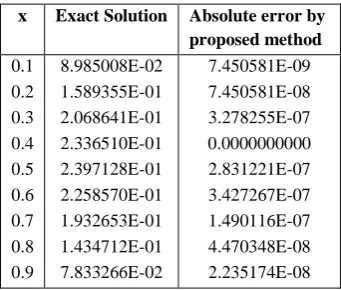
The exact solution for the above problem is y= (1-x) sin x. The proposed method is tested on this problem where the domain [0, 1] is divided into 10 equal subintervals. The obtained numerical results for this problem are given in Table 3. The maximum absolute error obtained by the proposed method is 3.427267x10⁻⁷.
Table 3: Numerical results for Example 3
x Exact Solution Absolute error by
proposed method
0.1 0.2 0.3 0.4 0.5 0.6 0.7 0.8 0.9
8.985008E-02 1.589355E-01 2.068641E-01 2.336510E-01 2.397128E-01 2.258570E-01 1.932653E-01 1.434712E-01 7.833266E-02
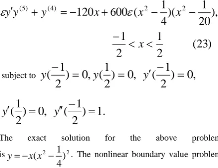
[image:4.595.343.514.599.744.2]Example 4: Consider the nonlinear boundary value problem
)
23
(
2
1
2
1
),
20
1
)(
4
1
(
600
120
2 2) 4 ( ) 5 (
x
x
x
x
y
y
y
subject to
)
0
,
2
1
(
,
0
)
2
1
(
,
0
)
2
1
(
y
y
y
.
1
)
2
1
(
,
0
)
2
1
(
y
y
The exact solution for the above problem
is 2 2
)
4
1
(
x
x
y
. The nonlinear boundary value problem(23) is converted into a sequence of linear boundary value problems generated by quasilinearization technique [19] as
,
120
)
20
1
)(
4
1
(
600
2 2) ( ) 5 (
) ( ) 1 ( ) 5 (
) ( )
4 (
) 1 ( )
5 (
) 1 ( ) (
x
x
x
y
y
y
y
y
y
y
n n n n n n n
n=0, 1, 2, …. (24)
subject to
)
0
,
2
1
(
,
0
)
2
1
(
( 1)) 1
(
n
n
y
y
.
1
)
2
1
(
,
0
)
2
1
(
,
0
)
2
1
(
( 1) ( 1)) 1
(
ny
ny
ny
Here y(n+1) is the (n+1) th
approximation for y. The domain
]
2
1
,
2
1
[
is divided into 10 equal subintervals and theproposed method is applied to the sequence of linear problems (24). The obtained numerical results for this problem with
01
.
0
[image:5.595.55.276.92.262.2]
are presented in Table 4. The maximum absolute error obtained by the proposed method is 1.569279x10⁻⁷.Table 4: Numerical results for Example 4
x Exact Solution Absolute error by
proposed method
-0.4 -0.3 -0.2 -0.1 0.0 0.1 0.2 0.3 0.4
3.240000E-03 7.680000E-03 8.820000E-03 5.760000E-03 0.0000000000 -5.760001E-03 -8.820000E-03 -7.680000E-03 -3.240000E-03
1.569279E-07 2.095476E-08 8.847564E-08 5.727634E-08 5.945729E-08 5.820766E-08 5.587935E-09 8.800998E-08 1.240987E-07
6.
CONCLUSIONS
In this paper, a Galerkin method with quartic B-splines as basis functions has been developed to solve a general fifth order boundary value problem. The quartic B-spline basis set has been redefined into a new set of basis functions which vanish on the boundary where the Dirichlet boundary conditions and Neumann boundary conditions are prescribed. The proposed method has been tested on three linear boundary value problems and a nonlinear fifth order boundary value problem. The numerical results obtained by the proposed method are in good agreement with the exact solutions available in the literature. The objective of this paper is to present a simple and efficient method to solve a general fifth order boundary value problem.
7.
REFERENCES
[1] Davies, A. R., Karageorghis., and Phillips. Spectral Galerkin Methods for the primary two point boundary value problem in modeling viscoealastics flows. International Journal of Numerical Methods in Engineering. 26 (1988), 647-662.
[2] Davies, A. R., Karageorghis., and Phillips. Spectral Collocation Methods for the primary two point boundary value problem in modeling viscoealastics flows. International Journal of Numerical Methods in Engineering. 26 (1988), 805-813.
[3] Agarwal, R. P. 1986 Boundary value problems for higher order differential equations. World Scientific, Singapore.
[4] Fyfe, D. J. Linear dependence relations connecting equal interval Nth degree splines and their derivatives. Journal of the Institute of Mathematics and its Applications. 7 (1971), 398-406.
[5] Shahid, S. Siddiqi., Ghazala, Akram., and Arfa, Elahi. 2008. Quartic spline solutions of linear fifth order boundary value problems. Applied Mathematics and Computation. 196 (2008), 214-220.
[6] Shahid, S. Siddiqi., and Ghazala, Akram. Sextic spline solutions of fifth order boundary value problems. Applied Mathematics Letters. 20 (2007), 591-597.
[7] Shahid, S. Siddiqi., and Ghazala, Akram. Solution of fifth order boundary value problems using non-polynomial spline technique. Applied Mathematics and Computation. 175 (2006), 1574-1581.
[8] Rashidinia, J., Jalilian, R., and Ghasemi, M. An O(h6) numerical solution of general nonlinear fifth order two point boundary value problems. Numerical Algorithms. 55 (2010), 403-428.
[9] Rashidinia, J., Jalilian, R., and Farajeyan, K. Non-polynomial spline approach to the solution of fifth-order boundary value problems. Journal of Information and Computing Science. 4 (2009), 265-274.
[10] Hikmet, Caglar., Nazan, Caglar., and Twizell. The numerical solution of fifth order boundary value problems with sixth degree B-spline functions. Applied Mathematics Letter. 12 (1999), 25-30.
[12] Feng-Gong, Lang., and Xiao-Ping, Xu. A new cubic B-Spline method for linear fifth order boundary value problems. Journal of Computational and Applied Mathematics. 36 (2011), 101-116.
[13] Feng-Gong, Lang., and Xiao-Ping ,Xu. Quartic B-Spline Collocation method for fifth order boundary value problems. Computing. 92 (2011), 365-378.
[14] Lamnii, A., Mraoui., and Tijini, A. Sextic spline solution of fifth-order boundary value problems. Mathematics and Computers in Simulation. 77(2008), 237-246.
[15] Kasi, Viswanadham, K. N. S., and Murali, Krishna, P. Quintic B-splines Galerkin for fifth order boundary value problems. ARPN Journal of Engineering and Applied Sciences. 5(2010), 74-77.
[16] Kasi, Viswanadham, K. N. S., and Showri, Raju, Y. Cubic B-spline Collocation method for fifth boundary value problems. International Journal for Mathematical Sciences and Engineering Applications. 6(2012), 431-447.
[17] Kasi, Viswanadham, K. N. S., and Showri, Raju, Y. Quartic B-spline Collocation method for fifth boundary value problems. International Journal of Computer Applications. 3 (2012), 1-6.
[18] Kasi, Viswanadham, K. N. S., Murali, Krishna, P., and Prabhakara, Rao, C. Numerical solution of fifth order boundary value problems by Collocation method with sixth order B-splines. International Journal of Applied Science and Engineering. 8 (2010), 119-125.
[19] Bellman, R. E., and Kalabaa, R. E., 1965 Quasilinearzation and Nonlinear boundary value problems. American Elsevier, New York.
[20] Bers, L., John, F., and Schecheter, M. 1964 Partial differential equations. John Wiley Inter Science, New York.
[21] Lions, J. L., and Magenes, E. 1972 Non-Homogeneous boundary value problem and applications. Springer-Verlag, Berlin.
[22] Mitchel, A. R., and Wait, R. 1977 The finite flement method in partial differential equations. John Wiley and Sons, London.
[23] Prenter, P. M. 1989 Splines and variational methods. John Wiley and Sons, New York.
[24] Carl, de-Boor, 2001 A pratical guide to splines. Springer-Verlag.