Scientific research measures

Full text

(1)Scientific Research Measures Marco Frittelli∗ Department of Mathematics University of Milan Loriano Mancini† Swiss Finance Institute at EPFL Ilaria Peri‡ ESC Rennes School of Business January 29, 2015. ∗Marco Frittelli, Department of Mathematics, University of Milan, Via Saldini 50, I-20133 Milan, Italy. E-mail: [email protected]. †Loriano Mancini, College of Management, EPFL, Quartier UNIL-Dorigny, CH-1015 Lausanne, Switzerland. E-mail: [email protected]. ‡Ilaria Peri, Finance and Operations Department, ESC Rennes, 2 rue Robert d’Arbrissel CS 76522, F-35065 Rennes Cedex, France. E-mail: [email protected].. Abstract The evaluation of scientific research is crucial for both the academic community and society as a whole. Numerous bibliometric indices have been proposed for the ranking of research performance, mainly on an ad hoc basis. We now introduce the novel class of Scientific Research Measures (SRMs) to rank scientists’ research performance and provide a rigorous theoretical foundation for these measures. In contrast to many bibliometric indices, SRMs take into account the whole citation curve of the scientist, offer appealing structural properties, allow a finer ranking of scientists, correspond to specific features of different disciplines, research areas and seniorities, and include several bibliometric indices as special cases. Thus SRMs result in more accurate rankings than ad hoc bibliometric indices. We also introduce the further general class of Dual SRMs that reflect the “value” of journals and permit the ranking of research institutions based on theoretically sound criteria, which has been a central theme in the scientific community over recent decades. An empirical application to the citation curves of 173 finance scholars shows that SRMs can be easily calibrated to actual citation curves and generate different authors’ rankings than those produced by seven traditional bibliometric indices.. Keywords: Research Performance, Scientific Impact Measures, Bibliometric Indices, Citations, Calibration JEL Codes: C02, I20 1.

(2) Introduction Over the last decades, the evaluation of scientific research performance has become increasingly important. Crucial decisions such as the funding of research projects or faculty recruitment depend to a large extent upon the scientific merits of the researchers involved. The selection of inappropriate valuation criteria can have deleterious effects on the performance assessment of scientists and structures, such as departments or laboratories, distort funding allocation and recruiting processes, and ultimately have a negative impact on society as a whole. Two approaches have been proposed to assess research performance: peer review valuation, based on internal committees and external panels of reviewers, and bibliometric valuation, based on bibliometric indices, i.e., statistics derived from the citations and characteristics of journals in which the research output appeared. Peer review valuation can only be carried out on a multiple-year basis and used to check or fine-tune the evaluation based on citation indices. In contrast, bibliometric valuation is far less expensive in terms of time and resources and can easily be carried out on a systematic, e.g., yearly, basis. Moreover, bibliometric valuation is essentially the only viable method when a large number of scientists or research outputs have to be evaluated. Because of the rapid increase in availability and quality of online databases (e.g., Google Scholar, Thomson Reuters’ Web of Science, Scopus, MathSciNet), bibliometric valuation has become widely popular and numerous bibliometric indices have been proposed to assess research performance. The most popular citation-based metric is the h-index introduced by Hirsch (2005). The h-index is the largest number such that h publications have at least h citations each. This index has received a great deal of attention from the scientific community and been widely used to assess research performance in many fields, e.g., Bornmann and Daniel (2007). Various authors have recently proposed several extensions of the h-index, mainly on an ad hoc basis, to improve on some of its shortcomings.1 This paper provides three contributions to the fast-growing literature on research valuation. The first contribution is to introduce a novel class of scientific performance measures designated Scientific Research Measures (SRMs). The main features of SRMs are that they take into account the scientist’s whole citation curve2 and rank research performance using a novel tool designated performance curves for research performance, similar to isotherm lines for temperature. Importantly, performance curves can be chosen in a flexible way, reflecting the scientists’ seniority and characteristics of the research fields, such as typical number of publications and citation rates. This flexibility is lacking in virtually all existing bibliometric indices. SRMs are derived from a “calibration” approach in the sense that they are informed by actual citation data. The second contribution of this paper is to introduce a further general class of research measures designated Dual SRMs. We provide a rigorous theoretical foundation for Dual SRMs building on the well-established theory of risk measures.3 Dual SRMs are rooted in the most recent developments of this theory, leading to the notion of quasi-convex risk measures. 2.

(3) introduced by Cerreia-Vioglio, Maccheroni, Marinacci, and Montrucchio (2011) and further developed in the dynamic framework by Frittelli and Maggis (2011).4 Dual SRMs are relevant for three reasons. First, if two scientists have the same citation curve, any traditional bibliometric index is unable to rank them, whereas Dual SRMs can rank those scientists as soon as their publications appear in different journals. Second, additional information, such as journals’ impact factors, can be taken into account in a theoretically consistent manner in research rankings based on Dual SRMs. Third, and perhaps most importantly, Dual SRMs are able to achieve a meaningful aggregation of scientists’ research outputs. This in turn allows the ranking of the research performance of teams, departments and academic institutions using theoretically sound criteria. The issue of ranking research institutions has been a central theme in the scientific community over recent decades, e.g., Borokhovich, Bricker, Brunarski and Simkins (1995), Kalaitzidakis, Mamuneas and Stengos (2003), and Bornmann, Stefaner, de Moya Anegón and Mutz (2014). The third contribution of this paper is to present an extensive empirical application of SRMs. Using Google Scholar, we construct a novel data set of citation curves for 173 finance scholars affiliated to 11 major US finance departments. We observe that power law performance curves fit actual citation curves well. Therefore we compare research rankings based on the SRM characterized by power law performance curves with seven other existing bibliometric indices. We find that the rankings of authors and universities based on the SRM are quite different from those based on the other bibliometric indices. The largest discrepancies concern “average” performing scholars and universities (in relative terms) that are arguably the most difficult to rank. Under the premise that research performance is reflected by the whole citation curve rather than only part of it, SRMs provide a better ranking of research performance than traditional bibliometric indices. Finally, we develop a simple two-step algorithm to operationalize SRMs.. Related Literature Since the early nineties, the use of bibliometric indices has encompassed many fields, e.g., Chung and Cox (1990), May (1997), Hauser (1998), Wiberley (2003), and Kalaitzidakis et al. (2003). The effectiveness of citation-based metrics has been validated by correlation analyses with peer review ratings, e.g., Lovegrove and Johnson (2008). Moreover, when a large number of scientists or research outputs need to be evaluated, bibliometric indices are essentially the only viable method.5 Hirsch (2005) introduced the h-index, which is nowadays the most popular citation-based metric. The main achievement of the h-index is to combine the number of publications and the number of citations in a single bibliometric index. One limitation of the h-index is its insufficient ability to discriminate between scientists’ research performances. The h-index is fully determined by the Hirsch core, i.e., the set of the most cited publications with at least h citations each. While the h-index is insensitive to publications with high and low numbers of citations, these publications may well contain valuable information for ranking scientific performances. The report by the Joint Committee on Quantitative Assessment of Research 6 (Adler, Ewing, & Taylor, 2008) confirmed this point by a well-documented example and encouraged the use of more complex measures.7. 3.

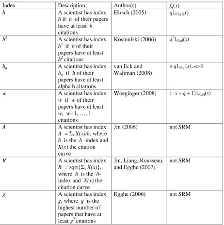
(4) To overcome the limitations of the h-index, a number of scientists from different fields have proposed a wide range of indices to measure scientific performances. We classify these numerous proposals into two broad categories: h-index variants, which suggest alternative methods to determine the core size of the most cited publications, and h-index complements, which include additional information in the h-index especially concerning the most cited publications. Among the h-index variants, one of the first proposals was the g-index by Egghe (2006). The g-index is defined as the largest number g such that the most cited g articles received at least g2 citations. Following the same logic, Kosmulski (2006) suggests the h2-index defined as the largest number h such that the h most cited publications receive at least h2 citations each. Compared to the h-index, the h2-index is probably more appropriate in fields where the number of citations per article is relatively high, such as chemistry or physics, while the hindex seems to be more appropriate for mathematics or astronomy for instance. Many studies point out the arbitrariness of the definition of the citation core size. To attenuate this problem, van Eck and Waltman (2008) propose the ha-index defined as the largest natural number ha such that the ha most cited publications receive at least a ha citations each. A further variant is the w-index introduced by Woeginger (2008), and defined as follows: a scientist has index w if w of their publications have at least w, w−1, . . . , 1 citations. Ruane and Tol (2008) propose the rational h-index (hrat-index) that has the advantage of providing more granularity in the evaluation process since it increases in smaller increments than the original h-index. Rousseau (2006, 2014) proposed the real (or interpolated) h-index, and Guns and Rousseau (2009) review several real and rational variants of the h- and g-indices. The h-index complements seek to measure the core citation intensity. For example, Jin (2006) proposed computing the average of the Hirsch core citations (A-index). Subsequently, to reduce the penalization of the best scientists receiving many citations, Jin, Liang, Rousseau, and Egghe (2007) modify the A-index by taking the square root of the Hirsch core citations (R-index). The same approach is used by Egghe and Rousseau (2008) but they consider as citation core only a subset of the Hirsch core (hw-index). Both the R- and hw-indicies can be very sensitive to only a few publications with many citations. In an attempt to make these indices more robust, Bornmann, Mutz, and Daniel (2008) propose calculating the median, rather than the mean, of the citations in the Hirsch core (m-index). The distribution of citations is often positively skewed, and the suggestion of using the median seems a sensible proposal. An interesting h-index complement is the tapered h-index, proposed by Anderson, Hankin, and Killworth (2008), which attempts to take into account all citations and not just those in the Hirsch core. As alternative, Vinkler (2009) proposes the π-index defined as one hundredth of the total citations obtained by the most influential publications, which are defined as the square root of the total publications ranked in decreasing order of citations. Zhang (2009) suggests a complementary index to the h-index to summarize the excess citations in the Hirsch core by taking their square root (e-index). Further proposals to attenuate the drawbacks of the h-index include the geometric mean of the h- and g-indicies (hg-index by Alonso, Cabrerizo, Herrera-Viedma and Herrera (2010)), and the geometric mean of the h- and m-indices (q2-index by Cabrerizo, Alonso, Herrera-Viedma and Herrera (2010)). The main conclusion that emerges from this literature review is that many bibliometric indices have been proposed to remedy specific issues related either to the core size of publications or to the impact of such core publications. Moreover, as pointed out by Schreiber (2010), many of these indices lead to very similar rankings. 4.

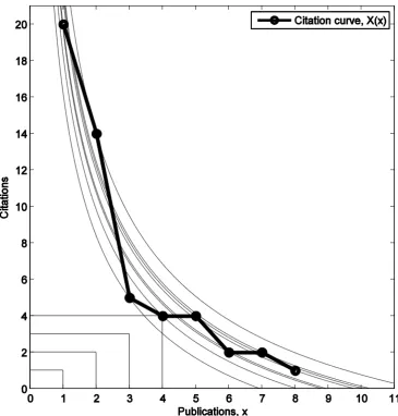
(5) Recently, Deineko and Woeginger (2009), Marchant (2009), and Ravallion and Wagstaff (2011) introduced new families of bibliometric indices, generalizing h-index type indices, using scoring rules, and using influence functions, respectively, in well-defined mathematical frameworks. We depart from the literature above by adopting a “calibration” approach, i.e., starting from observed citation curves, rather than improving existing bibliometric indices. The main motivation for our approach is that scientists of different fields and seniorities have significantly different citation curves. These differences are important and need to be reflected in the ranking process. Our SRMs take into account those specific features using flexible performance curves calibrated to actual data, as discussed in the next section.. Scientific Research Measures We now introduce the class of Scientific Research Measures. A scientist’s citation curve is the number of citations of each publication, in decreasing order of citations. Figure 1 shows a citation curve of a hypothetical scientist with eight publications. Insert Figure 1 here. We model the scientist’s citation curve, X, as a function X: R+ → R+, mapping each publication into the corresponding number of citations. By construction, X is bounded, nonincreasing, and non-negative. While the theory of SRMs holds when the domain and range of X are positive integers, we embed X in the positive reals for simplicity.8 To rank scientists’ research performances we introduce a new tool designated performance curves. The performance curve represents the amount of citations required to reach a performance level q. Intuitively, the higher the scientist’s research performance, the higher the performance curve fq that they can reach, and the higher the corresponding level q. Formally, the performance curve is a function fq : R+ → R that associates to each publication x a theoretical number of citations fq(x). The performance curve fq is assumed to be increasing in q, i.e., if q ≥ r then fq(x) ≥ fr(x) for all x. Although not necessary for the theory, we also assume that fq(x) is non-increasing in x, like any citation curve. When q varies in a given set I ⊆ R+, we obtain a family of performance curves {fq}q∈I. Typically, we will consider I = {1, 2, 3, . . .} ⊂ N or I = [1,∞]. Figure 1 shows two families of performance curves: square type functions corresponding to the h-index and power law type functions corresponding to a specific SRM that will be used in our empirical application. Moving from the origin (0, 0) of the graph in a northeasterly direction, the research performance level increases, i.e., each performance curve fq is associated to a higher and higher level q. The four performance curves in Figure 1 associated to the h-index correspond to an h-index of 1, 2, 3 and 4, respectively. Similarly, each power law type performance curve is associated to an increasing level of research performance. Our novel class of SRMs is defined by the following ϕ-index: ϕ(X) := sup{q ∈ I | X(x) ≥ fq(x), ∀x ∈ [1,∞)}. (1). 5.

(6) where := means defined as. The ϕ-index is obtained by comparing the whole citation curve X and the family of performance curves {fq}q∈I. Specifically, the ϕ-index is the highest level q of the performance curve still below the author’s citation curve. Consider again the power law type performance curves in Figure 1. The ϕ-index is 24.75 and determined by the performance curve passing through the point (3, 5). Generally speaking, numerical values of the ϕ-index have no interpretation and are simply used to rank scientists’ research performances. However, the ϕ-index can be normalized in order to interpret it.9 The family of performance curves {fq}q∈I plays a key role in the definition of SRMs. Performance curves create the common ground or “level the playing field” for the ranking of scientists’ research performances. The logic behind our approach is the following. Citation curves of researchers (with similar seniority) in a given field, say mathematics, tend to be quite similar. Across fields, however, say comparing mathematics and finance, the citation curves of researchers can be very different. In mathematics, researchers typically have a large number of publications with a small number of citations per publication. In finance, exactly the opposite happens. Thus different fields are characterized by different publication and citation practices. In our view these features of the research field, and seniority, should be reflected in the research ranking process, in a theoretically coherent manner. We propose to achieve this by calibrating performance curves to observed citation curves. Through statistical estimation, calibrated performance curves would then reflect the publication and citation practices in a given field. These performance curves vary across fields (area of research, seniority of researchers). A central feature of our method is that research performance is reflected by the whole citation curve, and not just part of it. We can illustrate this point with a simple example. Suppose two researchers, A and B, have a similar number of publications with similar citations, but researcher A has some additional, lightly cited publications compared to B. It appears that A should be ranked higher than B, but generally this ranking can be established only by considering the whole citation curves. In fact, if the additional, lightly cited publications of researcher A are disregarded, the two researchers would have very similar citation curves. Along similar lines, in many real cases it can be important to consider the whole citation curves in order to rank researchers correctly. Notice that by taking into account the whole citation curve, our ϕ-index does not necessarily penalize researchers with new or uncited publications. For example, if the eighth publication in Figure 1 had zero citations rather than one citation, the ϕ-index would not change. Under the premise that research performance is reflected by the whole citation curve, the issue is now to rank such curves. We tackle this by using our novel tool, namely the performance curves. Given that the citation curves of researchers of a given field and seniority are rather similar, it seems natural to us that performance curves should mimic the observed citation curves. These calibrated performance curves offer two advantages. First, as mentioned above, calibrated performance curves would reflect specific features of the field and seniority of researchers. Second, the calibration method is essentially an objective, data-driven procedure for the selection of performance curves, which is not significantly exposed to subjective or arbitrary judgments. When performance curves are not calibrated to observed citation curves, at least two issues may arise. The first is the arbitrariness in the selection of performance curves. These curves may have many shapes and it is a priori unclear which curves should be used to rank research 6.

(7) performance. As shown in our empirical application, different shapes of performance curves lead to different authors’ rankings, and the question remains as to which ranking should be used. The second is that arbitrarily chosen performance curves may not reflect important features of the research field and seniority of researchers. As already mentioned, performance curves in (1) can be specified in a flexible way, reflecting features of the scientific field, research areas, and seniority. Unfortunately most existing bibliometric indices lack such flexibility and their performance curves do not mimic observed citation curves. Figure 1 suggests that power law type performance curves mimic the citation curve X much better than square type performance curves do. As shown in our empirical application, observed citation curves exhibit power law shapes, calling for power law performance curves. While citation curves are always non-negative, the power law type performance curves in Figure 1 become negative for large x. This poses no problem to the ϕ-index and allows the taking into account of the scientist’s publications that have zero citations, i.e., those publications for which X(x) = 0.10 Monotonicity and Quasi-Concavity of SRMs The class of SRMs defined in (1) has two desirable properties: monotonicity and quasiconcavity. The first property simply indicates that better scientists, as reflected by their citation curves, have a higher ϕ-index. Formally, if Scientist 1 has a lower research performance than Scientist 2, i.e., X1 ≤ X2, then ϕ(X1) ≤ ϕ(X2). Thus, the monotonicity of the ϕ-index is well justified. If SRMs were characterized by monotonicity only, they would be of limited use. This is because the monotonicity property only allows the ranking of scientists whose citation curves satisfy a dominance order, like X1 ≤ X2. Evaluators often need to rank scientists whose citation curves intersect each other. The quasi-concavity of the ϕ-index enables scientists to be ranked in such more complex but realistic situations. Formally, quasi-concavity is expressed as follows: given two citation curves X1 and X2, quasi-concavity of the ϕ-index implies that, for all λ ∈ [0, 1], ϕ(λX1 + (1 − λ)X2) ≥ min(ϕ(X1), ϕ(X2)).. (2). Quasi-concavity indicates that a convex combination of two citation curves leads to a performance level which is at least as high as the research performance of the less well performing scientist. In other words, when the citation curve of a less well performing scientist is combined with the citation curve of a better performing scientist, the resulting research performance is at least as good as that of the less well performing scientist. This seems to be a natural property of the SRM. Appendix A shows that the ϕ-index in (1) satisfies (2), i.e., it is quasi-concave. Moreover, quasi-concavity ensures an internal consistency or coherency of scientists’ rankings and Appendix A provides a numerical example to illustrate this point. The appendix is available online at http://www.ssrn.com or from the authors upon request. Existing Bibliometric Indices as Scientific Research Measures. 7.

(8) The class of SRM defined in (1) includes many existing bibliometric indices. Different indices can be recovered by appropriately specifying the class of performance curves. For example the h-index is characterized by the performance curve fq(x) = q1(0,q](x), where 1(0,q](x) = 1 when x ∈ (0, q] and 0 otherwise. The performance curves of the real h-index are the same as those of the h-index but the q parameter varies in the real numbers. The maximum number of citations, as bibliometric index, is characterized by the performance curve fq(x) = q1(0,1](x). Similarly, the number of publications with at least one citation has performance curves given by fq(x) = 1(0,q](x). Table 1 shows the h2-, ha- and w-indices and their performance curves. Insert Table 1 here. Not all bibliometric indices proposed in the literature are SRMs. The ϕ-index in (1) has three features: it takes into account the whole citation curve, it is defined in terms of performance curves, and it is monotone and quasi-concave. Any bibliometric index that lacks any of these features is not an SRM. For example, the A-, R- and g-indices (defined in Table 1) are not SRMs since they do not take into account the scientist’s whole citation curve. Figure 2 shows six families of performance curves associated to six different bibliometric indices; see also Table 1. As citation curves have typically power law shapes, none of these performance curves provides an adequate description of actual citation curves. Insert Figure 2 here. Dual Scientific Research Measures We now introduce a further general class of research measures designated Dual SRMs. The goal is to reflect additional information in the ranking process in a theoretically consistent manner. We define a scientist’s citation record as the number of citations of publications in each journal. Dual SRMs rank citation records.11 Dual SRMs play the important role of allowing the aggregation of scientists’ research outputs in a meaningful way by aggregating citation records, namely the citations of publications of different scientists in the same journal. This in turn enables research teams, departments and academic institutions to be ranked in a theoretically sound way. The ranking of institutions has been a central theme in the scientific community over the last decades. We first provide a numerical example and then present the theory of Dual SRMs. Numerical Example of Dual SRMs To illustrate the derivation of the Dual SRM we use a simple numerical example. We consider an evaluator who seeks to rank scientists’ research performances. The first step is to select the evaluation criteria of the journals. The evaluator has to quantify the value of the journals in which the publications appeared. This is obviously a challenging task but is also a necessary step for ranking scientists with the same or similar distributions of citations, but with publications in different journals. Consider the following three journals: Management Science (MS), Mathematical Finance (MF), and Finance and Stochastics (FS). One possible way of assessing a journal’s value is to use the two-year and five-year journal’s impact factor.12 For MS, MF, and FS, the two-year 8.

(9) impact factors are 1.73, 1.25, and 1.15, and the five-year impact factors are 3.30, 1.66, and 1.58, respectively.13 The information expressed by each impact factor is collected in a probability measure, Q2 and Q5, respectively, on the journal space Ω = {MS, MF, FS}. For example, Q2(MS) = 1.73/(1.73 + 1.25 + 1.15), and similarly for the other journals and impact factors. Consider a scientist with three publications, one in each journal, MS, MF, and FS, with 10, six, and eight citations each. These citations are collected in their citation record X(ω), where ω = MS, MF, FS. Note that the citation record is not necessarily a citation curve, as the values of X(ω) need not be in decreasing order. In the current example these values are 10, six, and eight. The second step is to assess the scientist’s research performance relating to each criterion or probability measure Q2 and Q5. To that end, we introduce the function γ(Q2, m) that gives the smallest Q2-average of citations to reach a performance level of m. Intuitively, if the evaluator deems the criterion Q5 as highly important, then γ(Q5, m) will be high, and it will be a challenging task for each scientist to do well according to that criterion. If Q5 is more important than Q2, then γ(Q5, m) > γ(Q2, m). Hence, under Q2 the research performance of a scientist with citation record X(ω) is β(Q2,X) := sup{m ∈ R | EQ2[X] ≥ γ(Q2, m)}.. (3). Using citation record and impact factor, the value of EQ2[X] can be easily computed. In our example EQ2[X] = 10 Q2(MS) + 6 Q2(MF) + 8 Q2(FS) = 8.2. Suppose the evaluator has no preference between Q2 and Q5. Then γ(Q,m) can be set to a constant value, i.e., γ(Q, m) := m, for any Q, and thus β(Q2,X) := sup{m ∈ R | EQ2[X] ≥ m} = EQ2[X] = 8.2. If Q2 were the only criterion to assess journal quality, then β(Q2,X) = 8.2 was the scientist’s final research performance. Since Q5 is another criterion, the evaluator also computes the scientist’s research performance under Q5, obtaining a corresponding index of β(Q5,X). In our example EQ5[X] = 10 Q5(MS) + 6 Q5(MF) + 8 Q5(FS) = 8.5, and as γ(Q5, m) := m, then β(Q5,X) = EQ5[X] = 8.5. Finally, the evaluator takes the smaller value between β(Q2,X) and β(Q5,X). The Dual SRM gives the scientist’s final research performance Φ(X) := min(β(Q2,X), β(Q5,X)) = min(EQ2[X], EQ5[X]) = 8.2. This example shows that the Dual SRM leads to a conservative or “worst-case scenario” assessment of the research performance. The evaluator assesses the research performance using the least favorable journals’ evaluation criterion for the scientist. Generally, there will be no consensus on the journals’ evaluation criteria. Opting for a conservative assessment of research performance seems to be a sensible approach. To assess the research performance of another scientist, the evaluator repeats the steps above using the same Q2 and Q5 criteria. Comparing the scientists’ Φ-indices gives the scientists’ research rankings.. 9.

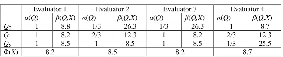
(10) Table 2 extends the numerical example above by introducing an additional journal evaluation criterion and considering four evaluators who assign different weights to the three criteria. The additional criterion is the number of years since the journal’s first edition expressed by the probability measure Q0.14 Under Q0, EQ0[X] = 10 Q0(MS) + 6 Q0(MF) + 8 Q0(FS) = 8.8. Insert Table 2 here. The evaluators’ decision to assign different weights to the three criteria can be expressed by choosing γ(Q, m) := m α(Q), where α(Q) ≥ 0 represents the weight that the evaluator assigns to criterion Q. The more important the criterion, the higher the α(Q). A natural range for the weights is the interval [0, 1] but weights larger than one are also admissible. If a particular criterion is controversial or deemed unimportant, it can be attributed a weight of zero. As in the initial example, for each evaluation criterion i = 0, 1, 5, β(Qi,X) := sup{m ∈ R | EQi[X] ≥ m α(Qi)} = EQi[X]/α(Qi) and the scientist’s final research performance Φ-index is Φ(X) := min(β(Q0,X), β(Q2,X), β(Q5,X)) = min(EQ0[X]/α(Q0), EQ2[X]/α(Q1), EQ5[X]/α(Q5)). Theoretical Derivation of Dual SRMs We now present a theoretical derivation of the Dual SRM. Formally, the citation record is a random variable X(ω) defined on the events ω ∈ Ω, where each event ω corresponds to the journal in which the publication appeared, and Ω is the set of journals. Thus, X(ω) is the number of citations of the publications in journal ω.15 We fix a family of probabilities P defined on Ω, where for each Q ∈ P, Q(ω) represents the value of journal ω ∈ Ω. A priori there will be no consensus regarding how journals are evaluated and this is reflected in the set Q ∈ P rather than just a single probability measure. We then select a family of functions {γ(Q, m)}m∈R. Each function γ(· , m) : P → R associates to each measure Q the value γ(Q, m), i.e., the smallest Q-average of citations to reach a research performance level m under Q. The Dual SRM is given by the Φ-index Φ(X) := inf β(Q,X) Q∈P. (4). where β(Q,X) := sup{m ∈ R | EQ[X] ≥ γ(Q, m)} represents the research performance of a scientist with citation record X, under the fixed measure Q. The function γ(Q, m) does not depend on the scientist’s citation record X and is non-decreasing in m. Any Dual SRM in (4) is monotone increasing and quasi-concave, as proved in Proposition 2 in Appendix B. The appendix is available online at http://www.ssrn.com or from the authors upon request. Both properties have a clear motivation. The monotonicity indicates that better scientists have higher research performances. The quasi-concavity indicates that the 10.

(11) performance of a research team is at least equal to the scientific performance of the less well performing member. Notably, quasi-concavity leads to sound rankings of research teams and institutions. This is because the citation records of two (or more) scientists can be aggregated by simply taking a linear convex combination λX1 + (1 − λ)X2, where λ ∈ [0, 1].16 The aggregation is meaningful since it is at the level of citation records, i.e., scientists’ citations of publications in the same journal. An important question is: Does any monotone increasing and quasi-concave map admit the representation in (4)? Essentially, the answer is positive and formalized in Theorem 1. To prove the theorem we assume the continuity from above of Φ and introduce some new notations. Let P be a probability measure defined on Ω. Since the citation record of an author X is a bounded function, it seems natural to take X ∈ L∞, where L∞ is the space of functions that are P almost surely bounded. We also denote with Δ:= {Q ≪ P} the set of all probabilities that are absolutely continuous with respect to P. Theorem 1 Any map Φ : L∞ → R that is quasi-concave, monotone increasing and continuous from above can be represented as Φ(X) := inf β(Q,X), ∀X ∈ L∞ Q∈Δ. (5). where β : Δ × L∞ → R and γ : Δ × R → R are defined as β(Q,X) := sup {m ∈ R | EQ[X] ≥ γ(Q, m)} γ(Q, m) := inf {EQ[Y] | Φ(Y ) ≥ m} . Y ∈L1. (6). The proof is provided in Appendix B.17 There are two technical differences between the ϕ-index in (1) and the Φ-index in (4). Remember that a law invariant function associates the same value to random variables with the same distribution law. The first difference is that the ϕ-index is law invariant while the Φindex may not be law invariant. In other words, if two scientists have the same citation curve, they have the same ϕ-index. If they publish in different journals, they generally have different Φ-indices. Thus, the Φ-index can rank scientists with the same citation curves, but who publish in different journals.18 The second difference is that the ϕ-index is not necessarily quasi-concave on the citation records (even if it is always quasi-concave on the citation curves). When the ϕ-index is quasi-concave on the citation records, the Φ-index includes the ϕ-index as a special case. Finally, note that if we endow the space L∞ with the weak topology σ(L∞, L1), its dual space is L1.. Empirical Analysis This section provides an empirical application of our SRM, discusses its implementation, and compares the empirical findings to those of seven existing bibliometric indices.19 11.

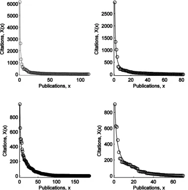
(12) Data We consider 173 full professors affiliated to 11 major US business schools or finance departments. The set of researchers is quite large and homogenous in terms of seniority and research field, making comparison significant. A Python script is run to extract their citation curves from Google Scholar (http://scholar.google.com/). Our data set is created on September 6, 2012. While entries in Google Scholar may suffer from data errors like any other database, the American Scientist Open Access Forum (2008) remarked that “Google Scholar’s accuracy is growing daily, with growing content.”20 Citation curves in Google Scholar are publicly and freely available. Our SRMs are not tailored to Google Scholar and can be applied to any other data set. Table 3 shows the list of business schools or finance departments that for brevity we call universities. The number of faculty members varies significantly across universities, ranging from eight members at Berkeley and Cornell to 34 members at Columbia. Table 3 also reports summary statistics for the number of citations and publications, aggregated at university level. Chicago has the largest average number of citations, as well as median and standard deviation, and fourth largest faculty by size. For all universities, the average number of citations is more than twice the median number of citations, suggesting that the distribution of citations is highly positively skewed. Princeton has the largest number of publications, and fifth largest faculty size. Insert Table 3 here. Estimates of the Scientific Research Measure To accurately rank research performance, performance curves should mimic actual citation curves. As all citation curves in our data set display power law shapes, we fit the power law function fq(x) = q/xc − k to each author’s citation curve.21 All estimated parameters are highly significant and adjusted R2’s are above 95%.22 As an example, Figure 3 shows four citation curves and fitted power law functions. Insert Figure 3 here. We use the following ϕ-index to rank authors: ϕ(X) := sup {q ∈ R | X(x) ≥ q/xc − k, ∀x ∈ [1,∞)}. (7). where c = 0.59 and k = 543.2, which are the weighted averages of all estimated c and k coefficients, respectively, with weights given by the number of data points used to estimate each coefficient.23 The following two-step algorithm can be used to compute the ϕ-index in (7). For each author: 1. Compute qx:= (X(x) + k) xc, for x = 1, 2, . . . , p, and q∗ := k pc 2. Take ϕ(X):= min(q1, q2, . . . , qp, q∗) where p is the number of publications with at least one citation. The performance curve associated to qx passes through the point (x, X(x)). This holds true for each x = 1, 2, . . . , p.24 The performance curve associated to q∗ crosses the horizontal axis at (p, 0), i.e., fq∗ (p) = 0. 12.

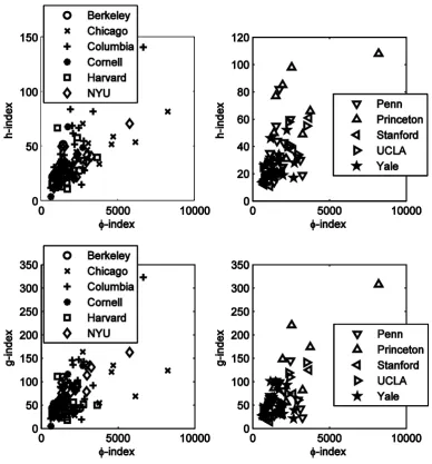
(13) This performance curve is considered because the whole citation curve may lie above the performance curve fq∗ and in that case fq∗ determines the ϕ-index in (7).25 To better understand the two-step algorithm, consider again Figure 1. This figure shows the p = 8 performance curves associated to q1, . . . , qp. The performance curve associated to q∗ is not shown but would pass through the point (8, 0). Taking the minimum of all the qx’s and q∗ (which is q3 = 24.75) ensures that the associated performance curve is below all the other performance curves (as performance curves are increasing in q), and consequently it is also below the citation curve X(x). At the same time, it is also the highest performance curve below the citation curve because it touches the citation curve at one point (which is (3, 5) in Figure 1). Empirical Results For each of the 173 authors in our data set, we compute the ϕ-index in (7) and the other seven bibliometric indices listed in Table 1. To provide an overview of the results, we aggregate estimates of the ϕ-index and bibliometric indices at the university level. Table 4 shows the mean and median for each index and university. Averages are often significantly larger than medians (e.g., for Princeton and Stanford), indicating that the distribution of the indices is positively skewed. Aggregate results should thus be interpreted cautiously. The main message from Table 4 is that rankings of universities based on our ϕ-index and the other bibliometric indices are generally different. Under the premise that research performance is reflected by the whole citation curve rather than only part of it, our ϕ-index provides a more accurate ranking of research performances than the other bibliometric indices. Differences in rankings are more concentrated on “average” performing universities, rather than best and least well performing universities, in relative terms. For example, according to the average ϕ-index, Chicago ranks first and Princeton second. According to the average h-index, Princeton ranks first and Chicago second. Berkeley ranks tenth according to both averages. For the remaining universities, the rankings provided by the ϕ- and h-indices, as well as the other indices, are quite different. Insert Table 4 here. Empirical results at the level of individual professors parallel the empirical results at university level. Owing to space constraints, we cannot report the estimates of all indices for all 173 full professors. To give some indication of the empirical findings, Figure 4 shows the scatter plots of the ϕ-index versus the h-index and versus the g-index for each scholar in our sample.26 The relationship between the indices is clearly positive. Best performing scholars tend to have the largest ϕ-, h-, and g-indices. Scholars in the top right-hand corner of the scatter plots are typically Nobel laureates in economics. This obviously results in a positive correlation between the indices. However, the relationship is far from monotone, meaning that different indices lead to different rankings. A closer look at the scatter plots reveals that various scholars have the same (or almost the same) h-index, while ϕ-indices are always different. Thus, the h-index cannot be used to rank them, while the ϕ-index provides a more granular ranking. This situation tends to occur when two authors have roughly the same number of publications but one author has more citations per publication, especially in the Hirsch core, and therefore a higher ϕ-index. In our data set, nine authors have an h-index of 21, nine authors of 25, and eight authors of 28. Thus, using 13.

(14) the h-index, 26 authors, i.e., 15% of all authors in our data set, would fall into three broad ranks, effectively not ranking them. All authors have a different ϕ-index. To summarize, this empirical application shows that our ϕ-index can be easily implemented and leads to different rankings from those of other bibliometric indices. Insert Figure 4 here. Conclusion The funding of research projects, faculty recruitment, and other key decisions for universities and research institutions depend to a large extent upon the scientific merits of the researchers involved. To rank scientists’ research performances, this paper introduces the novel class of Scientific Research Measures. The main feature of SRMs is that they take into account scientists’ whole citation curves as well as specific features of the scientific field, research areas, and seniority of scientists. This is achieved using flexible performance curves, whereas most existing bibliometric indices lack such flexibility. We also introduce the further general class of Dual SRMs to obtain more informed research rankings. Dual SRMs permit the aggregation of scientists’ research outputs and therefore theoretically result in well-founded rankings of research teams, departments and universities, something that has constituted a central theme in the scientific community over the last decades. Finally, we provide an empirical application using a novel data set of 173 finance scholars’ citation curves. Empirical results show that power law performance curves fit actual citation curves well. We find that authors’ rankings based on the SRM characterized by power law performance curves, and those produced by seven other bibliometric indices, are quite different. Under the premise that research performance is reflected by the whole citation curve, rather than only part of it, the SRM provides a more judicious ranking of research performances.. 14.

(15) Notes 1. For a review of these proposals, see e.g., Alonso, Cabrerizo, Herrera-Viedma and Herrera (2009), Panaretos and Malesios (2009), and Schreiber (2010). 2. The citation curve is the number of citations of each publication, in decreasing order of citations. 3. The axiomatic approach developed in the seminal paper by Artzner, Delbaen, Eber and Heath (1999) has been very influential for the theory of risk measures. Rather than focusing on a specific measurement of risk due to financial positions (e.g., variance of asset returns), Artzner et al. (1999) proposed a class of measures satisfying coherent axioms. Ideally, each financial institution could select its own risk measure, provided it obeyed the coherent axioms. This approach made the selection of the risk measure more flexible and, at the same time, established a unified framework. In the same spirit, we introduce Dual SRMs to rank research performance, rather than financial risks. Föllmer and Schied (2002) and Frittelli and Rosazza Gianin (2002) extended the theory of (coherent) risk measures to the class of convex risk measures. 4. Other studies in this area include Cherny and Madan (2009) who introduce the concept of an acceptability index having the property of quasi-concavity, and Drapeau and Kupper (2013) who analyze the relationship between quasi-convex risk measures and the associated family of acceptance sets, already present in Cherny and Madan (2009). 5. The Italian National Agency for the Evaluation of Universities and Research Institutes (ANVUR) is currently undertaking a large-scale evaluation process requiring the assessment of more than 200,000 research items (journal articles, monographs, book chapters, etc.) published by all Italian researchers between 2004 and 2010 in 14 different fields. Each panel, one for each field, consists of 30 members and has approximately 15,000 research items to evaluate in less than one year. All panels, except those in humanistic areas, decided to use bibliometric indices. 6. See http://www.mathunion.org/fileadmin/IMU/Report/CitationStatistics.pdf.. 7. Like any bibliometric index, the h-index presents other limitations concerning for example the issue of self-citations, the number of co-authors and the accuracy of bibliometric databases. Recently, various indices have been proposed to reduce these limitations. However, these indices are based on transformations of the original citation data, raising new issues concerning the best practice of carrying out such transformations. 8. As the number of publications and citations are positive integers, the domain and range for X appear to be the positive integers. However, in the research evaluation process, the domain and range of X need not be the positive integers. For example, if a publication is co-authored by two or more scientists, the evaluator may choose to count that publication as half or 1/(number of co-authors), when ranking the research performance of one of the co-authors. The evaluator may also choose to attribute more weight to citations of research papers, rather than review papers or books, making the range of X positive reals, rather than positive integers.. 15.

(16) 9. The performance curves in Figure 1 are given by fq(x) = q/xc−k. An equivalent representation of these performance curves is fq(x) = αq/xc−k. The parameter α can be used, for example, to normalize to 100 the ϕ-index of the scientist with the largest number of publications or citations, or any other scientist. This normalization is achieved by replacing q by αq in the two-step algorithm developed in the section “Estimates of the Scientific Research Measure” and determining α using the citation curve of the scientist with the largest number of publications or citations. 10. We thank Michael Schreiber for providing this comment as well as other insightful comments throughout the paper. 11. To implement Dual SRMs a richer data set is needed including citations, in which journals publications appeared, and quality of the journals. Retrieving such data can be challenging but necessary if this information is to be reflected in research rankings. 12. Other criteria are obviously conceivable to assess journal quality, such as overall citations of the journal or acceptance rate of journal submissions. Such additional criteria can be easily taken in account in the Dual SRM. For illustration purposes, we consider only two impact factors for each journal in this example. 13. The impact factors were obtained from the website of each journal in 2012. The impact factor was devised in the mid-1950s by Eugene Garfield. See Garfield (2005) for a recent account of the impact factor. 14. The first editions of MS, MF and FS appeared in 1954, 1991 and 1996, respectively, and in 2012 this implied Q0(MS) = (2012 − 1954)/95 = 0.61, Q0(MF) = (2012 − 1991)/95 = 0.22 and Q0(FS) = (2012 −1996)/95 = 0.17. 15. Over the years any scientist may have published more than one paper in the same journal. A simple approach to take this case into account would be to consider the total number of citations of all publications in a given journal. Indeed, if the journal evaluation criterion, say Qi, does not change over time, the total number of citations per journal is the only relevant statistic when assessing the scientist’s research performance as EQi[X] is a linear operator. To simplify the discussion of Dual SRMs we implicitly adopted this approach in the current section. If however the journal evaluation criterion changes over time (e.g., the impact factor of the journal), the citations of publications in a given year can be evaluated using the journal evaluation criteria for that year. Hence, citations of publications in different years can be evaluated using different journal evaluation criteria. 16. If λ = 0.5, the convex combination is simply the arithmetic mean of the two citation records. To aggregate n scientists’ citation records one computes Σi λiXi, where Σi λi = 1 and λi ≥ 0 for all i. 17. In (5) the infimum is taken with respect to all probabilities in Δ, and not in a prescribed subset P ⊆ Δ. This must be the case, since in the theorem the map Φ is given a priory and only the objects that can be determined from Φ can appear in the representation (5). 18. Frittelli, Maggis and Peri (2014) provide a theoretical analysis of quasi-convex maps defined on distributions.. 16.

(17) 19. As discussed in the previous section, an empirical application of Dual SRMs requires a richer data set, including in which journal each author’s publications appeared and the values of those journals. We defer such an application to future work. 20. http://openaccess.eprints.org/index.php?/archives/417-Citation-Statistics-InternationalMathematical-Union-Report.html. 21. To estimate the power law function we use nonlinear least squares and minimize Σx (X(x) − fq(x))2 with respect to the parameters q, c and k, where p is the author’s number of publications with at least one citation. Starting values for the nonlinear minimization are obtained as follows. The function f ˜q(x) = q/xc is a restricted version of fq(x), imposing k = 0. As in the log-log space f ˜q(x) is linear in log(x), i.e., log(f ˜q(x)) = log(q) − c log(x), the two parameter estimates logˆ(q) and cˆ can be easily obtained by the least square regression of log(X(x)) on a constant and log(x), where x = 1, 2, . . . , p. Starting values for q, c and k are exp(logˆ(q)), cˆ and 0, respectively. 22. Estimation results are available from the authors upon request.. 23. We also used other values of c and k, such as the simple average of all estimated c and k coefficients. The empirical results remained largely unchanged and are available from the authors upon request. 24. For example, the performance curve associated to qp is fqp (x) = qp/xc −k. When evaluated at x = p, it gives fqp (p) = qp/pc − k = (X(p) + k) pc/pc − k = X(p), confirming that this performance curve passes through the point (p,X(p)). 25. This situation may occur when the citation curve is roughly linear and steep. Although this is unlikely, the performance curve associated to q∗ needs to be considered when computing the ϕ-index in (7). More specifically, as p is the number of publications with at least one citation, the citation curve at x = p is such that X(p) ≥ 1 > 0 = fq* (p). Thus the citation curve X(x) may lie above fq* (x) for all x. Given the shape of the performance curves in Figure 1, this situation can occur when the citation curve is steep and roughly linear. As the citation curve X(x) = 0 for all x > p and the performance curves are increasing in q, it is not necessary to consider citation curves for q > q∗. All these performance curves lie above fq*, and thus above X(x) = 0 at least for all x > p, and do not determine the ϕ-index. 26. Scatter plots of the ϕ-index versus the other bibliometric indices are not reported, but share similar patterns.. 17.

(18) References Adler, R., Ewing, J., & Taylor, P. (2009). Citation statistics. Statistical Science, 24, 1–14. Alonso, S., Cabrerizo, F.J., Herrera-Viedma, E., & Herrera, F. (2009). h-index: A review focused in its variants, computation and standardization for different scientific fields. Journal of Informetrics, 3, 273–289. Alonso, S., Cabrerizo, F.J., Herrera-Viedma, E., & Herrera, F. (2010). hg-index: A new index to characterize the scientific output of researchers based on the h- and g-indices. Scientometrics, 82, 391–400. American Scientist Open Access Forum, (2008). Comments to the citation statistics report. Citation Statistics: International Mathematical Union Report, U.S. Anderson, T.R., Hankin, R.K.S., & Killworth, P.D. (2008). Beyond the Durfee square: Enhancing the h-index to score total publication output. Scientometrics, 76, 577–588. Artzner, P., Delbaen, F., Eber, J.M., & Heath, D. (1999). Coherent measure of risk. Mathematical Finance, 9, 203–228. Bornmann, L., & Daniel, H.D. (2007). What do we know about the h-index?. Journal of the American Society for Information Science and Technology, 58, 1381–1385. Bornmann, L., Mutz, R., & Daniel, H.D. (2008). Are there better indices for evaluation purposes than the h-index? A comparison of nine different variants of the h-index using data from biomedicine. Journal of the American Society for Information Science and Technology, 59, 830–837. Bornmann, L., Stefaner, M., de Moya Anegón, F., & Mutz, R. (2014). Ranking and mapping of universities and research-focused institutions worldwide based on highly-cited papers: A visualization of results from multi-level models. Online Information Review, 38, 43–58. Borokhovich, K.A., Bricker, R.J., Brunarski, K.R., & Simkins, B.J. (1995). Finance research productivity and influence. Journal of Finance, 50, 1691–1717. Cabrerizo, F.J., Alonso, S., Herrera-Viedma, E., & Herrera, F. (2010). q2-index: Quantitative and qualitative evaluation based on the number and impact of papers in the Hirsch core. Journal of Informetrics, 4, 23–28. Cerreia-Vioglio, S., Maccheroni, F., Marinacci, M., & Montrucchio, L. (2011). Risk measures: Rationality and diversification. Mathematical Finance, 21, 743–774. Cherny, A., & Madan, D. (2009). New measures for performance evaluation. Review of Financial Studies, 22, 2571–2606. Chung, K.H., & Cox, R.A.K. (1990). Patterns of productivity in the finance literature: A study of the bibliometric distributions. Journal of Finance, 45, 301–309.. 18.

(19) Deineko, V.G., & Woeginger, G.J. (2009). A new family of scientific impact measures: The generalized Kosmulski-indices. Scientometrics, 80, 819–826. Drapeau, S., & Kupper, M. (2013). Risk preferences and their robust representation. Mathematics of Operations Research, 38, 28–62. Egghe, L. (2006). Theory and practise of the g-index. Scientometrics, 69, 131–152. Egghe, L., & Rousseau, R. (2008). An h-index weighted by citation impact. Information Processing and Management, 44, 770–780. Föllmer, H., & Schied, A. (2002). Convex measures of risk and trading constraints. Finance and Stochastics, 6, 429–447. Frittelli, M., & Maggis, M. (2011). Dual representation of quasiconvex conditional maps. SIAM Journal on Financial Mathematics, 2, 357–382. Frittelli, M., Maggis, M., & Peri, I. (2014). Risk measures on P(R) and value at risk with probability/loss function. Mathematical Finance, 24, 442–463. Frittelli, M., & Rosazza Gianin, E. (2002). Putting order in risk measures. Journal of Banking and Finance, 26, 1473–1486. Garfield, E. (2005). The agony and the ecstasy – the history and meaning of the journal impact factor. International Congress on Peer Review and Biomedical Publication. Chicago. Guns, R., & Rousseau, R. (2009). Real and rational variants of the h-index and the g-index. Journal of Informetrics, 3, 64–71. Hauser, J.R. (1998). Research, development, and engineering metrics. Management Science, 44, 1670–1689. Hirsch, J.E. (2005). An index to quantify an individual’s scientific research output. Proceedings of the National Academy of Sciences, 102, 16569–16572. Jin, B. (2006). h-index: An evaluation indicator proposed by scientist. Science Focus, 1, 8–9. Jin, B., Liang, L., Rousseau, R., & Egghe, L. (2007). The R- and AR-indices: Complementing the h-index. Chinese Science Bulletin, 52, 855–863. Kalaitzidakis, P., Mamuneas, T.P., & Stengos, T. (2003). Rankings of academic journals and institutions in economics. Journal of the European Economic Association, 1, 1346–1366. Kosmulski, M. (2006). A new Hirsch-type index saves time and works equally well as the original h-index. ISSI Newsletter, 2, 4–6. Lovegrove, B.G., & Johnson, S.D. (2008). Assessment of research performance in biology: How well do peer review and bibliometry correlate?. BioScience, 58, 160–164. May, R. (1997). The scientific wealth of nations. Science, 275, 793–796. 19.

(20) Marchant, T. (2009). Score-based bibliometric rankings of authors. Journal of the American Society for Information Science and Technology, 60, 1132–1137. Panaretos, J., & Malesios, C. (2009). Assessing scientific research performance and impact with single indices. Scientometrics, 81, 635–670. Ravallion, M., & Wagstaff, A. (2011). On measuring scholarly influence by citations. Scientometrics, 88, 321–337. Rousseau, R. (2006). Simple models and the corresponding h- and g-index. preprint. Rousseau, R. (2014). A note on the interpolated or real-valued h-index with a generalization for fractional counting. Aslib Journal of Information Management, 66, 2–12. Ruane, F., & Tol, R.S.J. (2008). Rational (successive) h-indices: An application to economics in the Republic of Ireland. Scientometrics, 75, 395–405. Schreiber, M. (2010). Twenty Hirsch index variants and other indicators giving more or less preference to highly cited papers. Annals of Physics, 522, 536–554. van Eck, N.J., & Waltman, L. (2008). Generalizing the h- and g-indices. Journal of Informetrics, 2, 263–271. Vinkler, P. (2009). The π-index: A new indicator for assessing scientific impact. Journal of Information Science, 35, 602–612. Wiberley, S.E. (2003). A methodological approach to developing bibliometric models of types of humanities scholarship. Library Quarterly, 73, 121–159. Woeginger, G.J. (2008). An axiomatic characterization of the Hirsch-index. Mathematical Social Sciences, 56, 224–232. Zhang, C.T. (2009). The e-index, complementing the h-index for excess citations. PLoS ONE, 4, e5429.. 20.

(21) Figure 1: Citation curve. The graph shows the citation curve of a hypothetical scientist with eight publications, as well as performance curves based on the h-index and ϕ-index. The citation curve is obtained by sorting publications in decreasing order of citations. Performance curves of the h-index are given by fq(x) = q 1(0,q](x), with q = 1, 2, 3, 4. Performance curves of the ϕ-index are given by fq(x) = q/x0.55−8.49, with each curve passing through a different point (x, X(x)), with x = 1, 2, . . . , 8. The hypothetical scientist has an h-index of four and ϕ-index of 24.75. The ϕ-index is determined by the performance curve passing through the point (3, 5). This performance curve is the highest curve still below the citation curve X and indeed 24.75/30.55 − 8.49 = 5.. 21.

(22) Figure 2: Performance curves of existing bibliometric indices. The graph shows six families of performance curves corresponding to six different bibliometric indices: h-index with performance curve fq(x) = q1(0,q](x) and q = 1, 2, . . . , 7; h2-index with performance curve fq(x) = q21(0,q](x) and q = 1, 2, 3; ha-index with performance curve fq(x) = αq1(0,q](x), α = 0.5 and q = 1, 2, . . . , 7; w-index with performance curve fq(x) = (−x + q + 1)1(0,q](x) and q = 1, 2, . . . , 7; maximum number of citations with performance curve fq(x) = q1(0,1](x) and q = 1, 2, . . . , 7; number of publications with at least one citation each with performance curve fq(x) = 1(0,q](x) and q = 1, 2, . . . , 7.. 22.

(23) Figure 3: Typical fit of citation curves. Each graph shows one citation curve X(x) (circles), i.e., the author’s citations in decreasing order of citations, where x = 1, . . . , p and p is the number of publications with at least one citation. Superimposed is the fitted power law curve fq(x) = q/xc − k. For each author, parameter estimates of the power law curve are obtained using nonlinear least squares, i.e., by minimizing Σx (X(x) − fq(x))2 with respect to q, c and k. All adjusted R2’s are above 97.4%.. 23.

(24) Figure 4: Scatter plots of ϕ-index versus h- and g-indices. Upper graphs: scatter plot of ϕ-index (horizontal axis) versus h-index (vertical axis). Lower graphs: scatter plot of ϕ-index (horizontal axis) versus g-index (vertical axis). These indexes are computed for each one of the 173 scholars in our data set and displayed according to the university to which the scholar belongs. The relationships between ϕ-index and h-index (respectively g-index) are not monotone. Thus rankings of scholars given by the ϕ-index and h-index (respectively g-index) are different. The data set of citations covers 173 full professors affiliated to business schools or finance departments of 11 main US universities. The data set was extracted from Google Scholar on September 6, 2012.. 24.

(25) Table 1 Index h. h2. ha. w. A. R. g. Description A scientist has index h if h of their papers have at least h citations A scientist has index h2 if h of their papers have at least h2 citations A scientist has index ha if h of their papers have at least alpha h citations A scientist has index w if w of their papers have at least w, w−1, …, 1 citations A scientist has index A = Σx X(x)/h, where h is the h -index and X(x) the citation curve A scientist has index R = sqrt{Σx X(x)}, where h is the hindex and X(x) the citation curve A scientist has index g, where g is the highest number of papers that have at least g2 citations. Author(s) Hirsch (2005). fq(x) q1(0,q](x). Kosmulski (2006). q21(0,q](x). van Eck and Waltman (2008). α q1(0,q](x), α>0. Woeginger (2008). (−x + q + 1)1(0,q](x). Jin (2006). not SRM. Jin, Liang, Rousseau, and Egghe (2007). not SRM. Egghe (2006). not SRM. Table 1: Bibliometric indices. This table lists popular bibliometric indices, a short description of each, and the author(s) who introduced the index. The h-, h2-, ha-, and w-indices are Scientific Research Measures (SRMs) as defined in (1). The last column provides the functional form of the corresponding performance curves, fq(x). The A-, R-, and g-indices are not SRMs.. 25.

(26) Table 2 Evaluator 1 Evaluator 2 α(Q) β(Q,X) α(Q) β(Q,X) Q0 1 8.8 1/3 26.3 Q1 1 8.2 2/3 12.3 Q5 1 8.5 1 8.5 Φ(X) 8.2 8.5. Evaluator 3 α(Q) β(Q,X) 1/3 26.3 1 8.2 1 8.5 8.2. Evaluator 4 α(Q) β(Q,X) 1 8.7 2/3 12.3 1/3 25.5 8.7. Table 2: Numerical example of Dual SRMs. The journal space Ω consists of three journals, Ω = {MS, MF, FS}. The scientist has three publications, one in each journal, with 10, six, and eight citations, respectively, i.e., their citation record X(ω) is given by X(MS) = 10, X(MF) = 6, and X(FS) = 8. To assess their research performance, each evaluator uses three criteria expressed by the probability measures Q0, Q2, and Q5. Criterion Q0 expresses the number of years since the journal’s first edition (the journal’s first edition for MS, MF, and FS is 1954, 1991, and 1996, respectively). Criterion Q2 expresses the two-year impact factor of the journal (the two-year impact factor for MS, MF, and FS is 1.73, 1.25, and 1.15, respectively). Criterion Q5 expresses the five-year impact factor of the journal (the five-year impact factor for MS, MF, and FS is 3.3, 1.66, and 1.58, respectively). Each evaluator assigns different weights α(Q) to the three criteria and thus uses a different SRM. For each criterion Q, β(Q,X) := sup{m ∈ R | EQ[X] ≥ γ(Q, m)}, where γ(Q, m) := m α(Q). The Dual SRM gives the final research performance as Φ(X) = min(β(Q0,X), β(Q2,X), β(Q5,X)).. 26.

(27) Table 3 Full Name Berkeley Haas School of Business Chicago Chicago Booth Columbia Columbia Business School Cornell Johnson Harvard Harvard Business School NYU Stern School of Business Penn. Wharton, Univ. of Pennsylvania Princeton Bendheim Center for Finance Stanford Graduate School of Business UCLA Anderson School of Management Yale Yale School of Management. Faculty 8. Avg 90. Citations Med 21. Std 179. Avg 85. Publications Med Std 61 61. 17. 279. 68. 562. 104. 85. 97. 34. 121. 40. 237. 101. 63. 108. 8 15. 72 152. 23 45. 142 283. 181 59. 82 44. 302 61. 26. 110. 27. 285. 81. 73. 44. 21. 138. 48. 267. 77. 52. 67. 13. 127. 37. 268. 207. 82. 271. 11. 131. 52. 226. 43. 31. 32. 9. 145. 39. 281. 81. 74. 36. 11. 161. 55. 333. 75. 54. 45. Total. 173. Table 3: Data set. The data set includes 173 full professors affiliated to business schools or finance departments of 11 main US universities. Faculty is the number of full professors for each university in our data set. For each author, the data set includes the number of publications with at least one citation each and the number of citations per publication, i.e., the citation curve. Avg, Med and Std are average, median and standard deviation, respectively, of citations and publications of all full professors for each university. Entries are rounded to the nearest integer. The data set of citations and publications is from Google Scholar and was extracted on September 6, 2012.. 27.

(28) Table 4 – Part 1 ϕ Avg Berkeley 1,504 Chicago 3,007 Columbia 1,778 Cornell 1,495 Harvard 1,705 NYU 1,768 Penn. 1,653 Princeton 2,404 Stanford 1,536 UCLA 1,962 Yale 1,726. Med 1,489 2,338 1,415 1,446 1,626 1,428 1,516 1,853 1,109 2,267 1,706. h Avg 27 41 38 32 28 33 31 51 23 37 30. Med 41 60 50 51 34 52 42 82 28 53 44. A Avg 185 479 229 171 247 238 235 296 219 286 274. Med 25 38 30 29 23 31 25 49 19 34 29. h2 Avg 10 16 12 10 11 12 11 14 11 13 12. Med 160 331 186 146 239 186 174 278 218 320 244. R Avg 69 135 88 73 79 85 79 119 70 100 85. Med 10 15 11 11 10 12 10 13 9 15 11. ha Avg 35 48 46 43 33 40 39 67 28 45 36. Med 32 42 36 36 26 38 32 62 20 40 33. Med 65 117 79 71 68 81 64 94 61 113 84. g Avg 56 83 73 69 48 71 58 106 43 76 59. Med 44 85 57 56 44 67 52 82 31 61 54. Table 4 – Part 2 w Avg Berkeley 47 Chicago 66 Columbia 63 Cornell 57 Harvard 45 NYU 57 Penn. 52 Princeton 91 Stanford 37 UCLA 63 Yale 49. Table 4: The Scientific Research Measure and bibliometric indices. For each scholar in our data set, ϕ-, h-, h2-, ha (with α = 0.5), w-, A-, R-, and g-index are computed. The ϕ-index is based on power law performance curves. For each index, Avg and Med are average and median of the index of all scholars in a given university. Entries are rounded to the nearest integer. The data set of citations covers 173 full professors affiliated to business schools or finance departments of 11 main US universities. The data set was extracted from Google Scholar on September 6, 2012.. 28.

(29)

No results found