BIROn - Birkbeck Institutional Research Online
Cooper, Richard P. (2016) Executive functions and the generation of
“Random” sequential responses:
a computational account.
Journal of
Mathematical Psychology 73 (1), pp. 153-168. ISSN 0022-2496.
Downloaded from:
Usage Guidelines:
Please refer to usage guidelines at or alternatively
To appear in the Journal of Mathematical Psychology Final draft. June 2016
Executive Functions and the Generation of “Random” Sequential Responses:
A Computational Account
Author: Richard P. Cooper
Affiliation: Centre for Cognition, Computation and Modelling Department of Psychological Sciences
Birkbeck, University of London
Telephone: +44 20 7631 6211
Email: [email protected]
Executive Functions and the Generation of “Random” Sequential
Responses: A Computational Account
Richard P. Cooper
Centre for Cognition, Computation and Modelling Department of Psychological Sciences
Birkbeck, University of London
Abstract: When asked to generate sequences of random responses, people exhibit strong and reliable biases in their behaviour. The origins of these biases have been linked to the operation of so-called executive functions through empirical studies varying, e.g., rate of production, modality of response, and (in dual task conditions) secondary task. We present a computational process model of random generation that accounts for a broad range of these empirical effects. The model, which operationalises a previous verbal account of random generation, is grounded in both the cognitive architectures and the executive functions literatures. As such, it instantiates a hypothesis concerning the interaction of multiple distinct executive functions in the generation of complex behaviour. In particular, it is argued on the basis of simulations of empirical findings that three cognitive factors play separable roles in random generation behaviour: cognitive load, which when high exacerbates underlying biases in a generation stage, monitoring, which when impaired results in greater inequality of response usage, and set-shifting, which when impaired results in less frequent switching between response schemas.
Highlights:
We present an information-processing model of random generation behaviour
The model is developed within a more general cognitive architecture
The architecture makes explicit the role of executive functions
The model reproduces random generation performance in single and dual task conditions
Dual task performance is accounted for via interference to executive control
Keywords:
Executive function; information processing model; random generation; set shifting; monitoring; response inhibition.
1
Introduction
Boucher, Palmeri, Logan & Schall, 2007; Wiecki & Frank, 2013). A limitation of much of this work – though one that is reasonable given the developing nature of the field – is that it generally considers the operation of individual executive functions in isolation on relatively simple executive function tasks. For example, the Boucher et al. (2007) model focuses on a version of the stop-signal task, in which a subject must, on a small proportion of trials normally signalled by a tone, withhold the production of an otherwise routine response such as a button press. Working at a similar level of complexity, Gilbert and Shallice (2002) focus specifically on the process of task set switching involved in switching from word reading to colour naming (and vice versa) in the Stroop task. While this work has advanced our understanding of basic executive functions, behaviour on tasks of greater complexity is likely to require multiple executive functions working in concert in order to appropriately regulate behaviour.
A landmark empirical study specifically aimed at understanding the role of executive functions in more complex tasks is the individual differences study of Miyake et al. (2000). These authors considered the correlational structure of the performance of over 130 individuals on 14 tasks, comprising 9 relatively simple tasks and 5 more complex tasks. The simple tasks included three held primarily to tap the putative executive function of set-shifting, three to tap memory updating and monitoring, and three to tap response inhibition. Subject performance within each subset of three simple tasks was found to correlate more highly than between subsets, as supported by Confirmatory Factor Analysis (CFA). The three factors obtained from this analysis were then used via Structural Equation Modelling (SEM) to determine the role of the three underlying constructs in the more complex tasks. Thus, on the basis of this it was argued that, for example, in the Wisconsin Card Sorting Test the set-shifting function (and this function alone) was critical in limiting the production of perseverative errors. This was in contrast to an alternative hypothesis, namely that such errors arose from a failure in response inhibition.
One of the five complex executive tasks used by Miyake et al. (2000) was random number generation. In random generation tasks, which are widely used in executive function research (e.g., Baddeley, Emslie, Kolodny & Duncan, 1998; Cooper, Wutke & Davelaar, 2012; Jahanshahi et al., 1998, 2000, 2006; Peters, Giesbrecht, Jelicic & Merckelbach, 2007; Proios, Asaridou & Brugger, 2008; Towse, 1998; Towse et al., 2016), subjects are asked to produce a sequence of “random” responses. More precisely, subjects are required to produce responses where each successive response is independent of his or her previous responses, or equivalently, where each successive response cannot be predicted with greater than chance accuracy from the subject’s previous responses. Random generation tasks typically yield multiple dissociable dependent measures (as discussed in detail below; see also Towse & Neil, 1998), and Miyake et al. argue on the basis of their SEM analysis that different dependent measures reflect the efficacy of different executive functions. This paper aims to evaluate the account of executive involvement in random generation performance given by Miyake et al. and, more generally, to explore the interaction of executive functions on a task with multiple dependent measures. We present a computational account of random generation derived from the verbal model of Baddeley et al. (1998) and grounded in a cognitive architecture in which executive functions have explicit roles. The model, which is a development of that of Sexton and Cooper (2014), is evaluated both against the results of Miyake et al. and against results from a dual task study of Cooper et al. (2012) where the primary task was random generation.
the verbal model of Baddeley et al. (1998), embedding it within a cognitive architecture based on the Contention Scheduling / Supervisory System approach of Norman and Shallice (1986). Critically, the Supervisory System part of the model draws also on the executive functions investigated by Miyake et al. (2000) and the decomposition of supervisory processes outlined by Shallice and Burgess (1996). Subsequent sections report simulation studies that demonstrate that the model can capture both frequently reported biases in random generation and the interference patterns arising from concurrent performance of different secondary tasks. The general discussion focuses on two broad sets of issues: the role of key parameters of the model and their relation to the efficacy of executive functions; and the model’s architecture as an elaboration of the verbal theories on which it is based, with a specific focus on the relationship between the model’s architecture and other established cognitive architectures (including ACT-R: Anderson, 1993, 2007, and Soar: Newell, 1990; Laird, 2012).
2
Random Generation
2.1 Dependent Measures and Standard Effects
Random generation tasks have a long history within information processing psychology research (see Tunes, 1964, and Wagenaar, 1972, for early reviews). Behaviour is typically assessed through measures of randomness calculated from the sequence of responses produced by the subject. The degree of randomness of a sequence cannot be characterised with a single measure and many different measures have been considered. Thus, if each successive response in a sequence is equally likely but independent of the previous responses then one would expect, over the long run, that each response would occur equally often. The degree of response equality is frequently quantified in information-theoretic terms by the redundancy, or R, score:
𝑅 = 100 × (1 −log2𝑛 −
1
𝑛 ∑ 𝑛𝑖 𝑖. log2𝑛𝑖
log2𝑎 ) (1)
where n is the number of responses in the sequence, a is the size of the response set, and ni is the number of times response i is produced.
The redundancy score, which is a linear transformation of the Shannon entropy (Shannon, 1948) of the multiset of elements in sequence, ranges from 0 to 100 and is 0 when each response is equally frequent and 100 when all responses are identical (i.e., when a single response is repeated).
A highly unpredictable sequence will have a low redundancy score, but cycling through all possible responses will similarly produce a low redundancy score. It is therefore necessary to also consider the relative frequency of response pairs (i.e., of bigrams). Again, in an ideal random sequence of infinite length each bigram should be equally frequent. Bigram equality may be quantified by calculating a redundancy score for bigrams (rather than individual responses) using equation 1. An alternative approach is the RNG score of Evans (1978):
𝑅𝑁𝐺 =∑ 𝑛𝑖𝑗 𝑖𝑗. log2𝑛𝑖𝑗 ∑ 𝑛𝑖 𝑖. log2𝑛𝑖
(2)
where ni is the frequency of response i
The RNG score scales the entropy of bigrams by the entropy of elements. It attains a maximum of 1 when an element is perfectly predicted by its predecessor (i.e., bigrams probabilities are zero or one). Lower values reflect greater equality of bigram usage. Note, however, that even if a sequence has perfect equality of bigram usage, it may still be predictable at the level of trigram (or higher) statistics. Further measures of randomness are therefore required. Indeed, Towse and Neil (1998) report 11 measures that have been used to quantify randomness, while Towse and Valentine (1997) consider 16.
The extensive empirical work on random generation has yielded several robust behavioural effects and substantial convergence on a verbal account of the underlying cognitive processes. With regard to the former, five findings in particular have been replicated by a number of studies:
1. Generation is more stereotyped when the response set is externally represented (e.g., subjects select from a visual array) than when the subject must hold the response set in mind (e.g., subjects select according to a criterion such as digits ranging from 1 to 10). See for example Baddeley et al. (1998) and Towse (1998), and see Wagenaar (1972) for a review of earlier studies.
2. Generation is affected by biases inherent in the response set or response modality (e.g., when responses are digits counting up/down is more likely than chance, when responses are letters associated letter pairs are more likely than chance, when responses are generated with keypads homologous finger selection on alternating hands is more likely than chance). See Baddeley (1966), Wiegersma (1984), Baddeley et al. (1998), Towse (1998) and Cooper et al. (2012).
3. Subjects produce far fewer repeat responses (e.g., “3” followed by “3” when generating digits) than would be expected if successive responses were independent. See, for example, Baddeley et al. (1998), Towse (1998), Cooper et al. (2012) and Towse et al. (2016).
4. Generation is more stereotyped when the response set is large (e.g., 15 items or more) than when it is small (e.g., 10 items or fewer). See Towse (1998) and Towse & Vallentine, (1997), and for a review of earlier work see Tunes (1964) and Brugger (1997).
5. When response generation is paced, responses are more stereotyped when response rate is fast (e.g., less than one per second) than slow (e.g., one per four seconds). See Baddeley (1966), Towse (1998) and Jahanshahi et al. (2000, 2006), and for a review of earlier work see Tunes (1964), Wagenaar (1972) and Brugger (1997).
Findings 2 and 3 relate specifically to biases in bigram production. In the other cases, R and RNG (where both are reported) generally behave analogously, with both showing a tendency towards increased stereotypy or predictability in the same conditions. However, R and RNG have also been shown to dissociate. For example, Towse and Valentine (1997) scored the randomly generated sequences of their subjects on 16 measures of randomness. They found considerable individual differences on these measures. Factor analysis suggested four dissociable factors underlying performance, which they labelled equality of response usage, prepotent associates, short repetitions, and long repetitions. The first of these correlates most strongly with R, while the second correlates more strongly with RNG and bigram measures (such as the adjacency index – an index of the relatively frequency of adjacent response pairs).
2.2 The Role of Executive Functions in Random Generation
updating” while prepotent associates was best accounted for by a model with one path from the executive construct of “response inhibition” (in both cases in contrast to models with paths from constructs related to task set shifting or memory updating and monitoring, or all three executive function constructs).
Cooper et al. (2012) argued that a potential limitation of the Miyake et al. (2000) study was its reliance on correlational rather than experimental methods. Miyake et al.’s conclusions from SEM analyses, in particular, depend on selecting the best structural model from a set of competing models, all of which have qualitatively similar fits. Cooper et al.’s approach was instead to consider interference on random generation due to different secondary tasks, where the secondary tasks were designed to tap different executive functions. Thus, when subjects attempted to generate sequences of random responses while concurrently completing the well-known 2-back task – a task held primarily to tap the putative executive function of memory monitoring and updating – the sequences so generated were far from random. In comparison to a baseline condition, the memory monitoring and updating task had a substantial inflationary effect on both R (reflecting decreased equality of response usage) and RNG (reflecting increased frequency of prepotent associates). A concurrent task designed to tap set-shifting – the digit-switching task of Monsell (2003) – had a similar substantial inflationary effect on R but a more modest effect on RNG. Finally, a concurrent task designed to tap response inhibition – a version of the popular go-no go task – had a modest inflationary effect on both R and RNG. Cooper et al. argued that the various patterns of interference in random generation, and in particular the dissociation between dependent measures occurring with the set-shifting task, reflected interference to different executive functions involved in the random generation task.
This apparent fractionation of executive function is important because it addresses a criticism sometimes levelled at theoretical accounts of executive function, namely that the oft-posited central executive is homuncular (e.g., Dennett, 1998). The existence of dissociable factors suggests dissociable processes underlying those factors, and hence that the central executive is not an atomic, non-decomposable, entity. Verbal accounts of the cognitive processes underlying random generation, as well as neuroscientific evidence, also support this position. Thus, Baddeley (1996; see also Baddeley et al., 1998) suggested that random generation involves a series of steps. Subjects, he suggests, use response schemas (like counting up by two, or down by one) to generate a putative response based on the previous response. This putative response is evaluated in the context of recent responses to determine whether it is “random”. If the putative response passes this evaluation, it is produced. Otherwise (and if time permits) the subject inhibits production of the putative response, switches to a new response schema, and generates a new putative response. While Baddeley did not elaborate this verbal account into a complete computational process model of random generation, it clearly draws on several distinct processes: one process to generate a putative response based on a previous response and a response schema; a monitoring process to evaluate whether the putative response is sufficiently random; and, if it is not, processes to suppress production of the putative response (i.e., a response inhibition process) and to generate or switch to an alternative response schema (i.e., a set shifting process). The model is therefore compatible with the Miyake et al. (2000) decomposition of executive processes.
terms of a model where left DLPFC provides top-down control that inhibits habitual schemas such as counting up or down by 1. A follow-up imaging study using PET was consistent with this interpretation (Jahanshahi et al., 2000).
2.3 A Re-examination of the Data of Cooper et al. (2012)
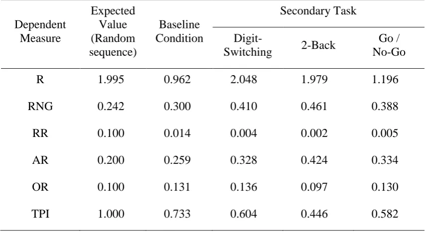
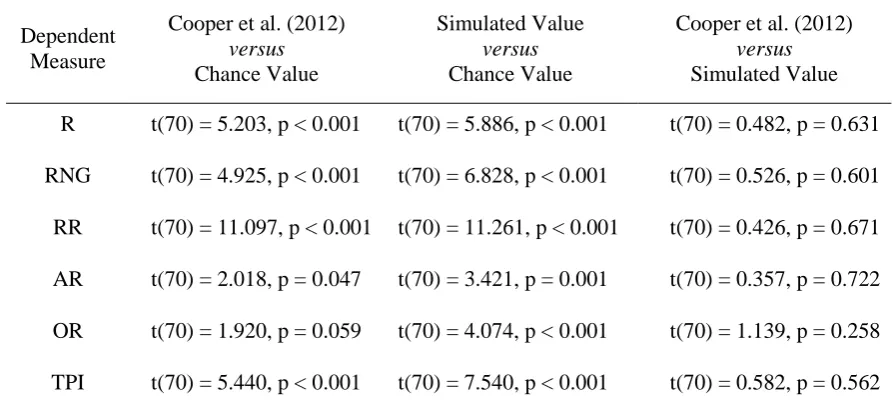
For the purposes of being concrete, this article considers in depth the random generation data from the dual-task study of Cooper et al. (2012). That study asked subjects to generate sequences of 100 responses selected using a computer mouse from a clock-face type display with 10 response options arranged around a central cursor. Selection was self-paced and the mouse automatically returned to the central cursor after each item was selected. The procedure was performed once with no secondary task and then three further times – once with each of three different secondary tasks (with secondary task order fully counterbalanced). Full details of the procedure are given in the original paper (Cooper et al., 2012). Key measures of randomness are reproduced in Table 1, where “expected values” are calculated from computer-generated pseudo-random sequences of 10 items and length 100.
Several aspects of the dataset are of note. First, while the expected value of R (cf. Equation 1) for an infinite sequence is zero, its expected value for finite sequences is greater than zero.1 Note also that the observed value of R in the baseline condition was less than the
1 To understand why, consider a sequence of 100 items with a response set of size 10 (as in the Cooper et al.,
[image:8.595.84.513.205.439.2]2012 study). R will have a value of zero if and only if the generated sequence contains exactly 10 instances of each response. In a random sequence this is highly unlikely. Suppose an agent is on target to produce such a sequence, and so after 99 responses all but one item has been produced 10 items, with the remaining item (say “A”) having been produced just 9 times. If responses are independent then there is clearly only a one in ten Table 1: Expected values of measures of randomness and their values from the dual-task study of Cooper et al. (2012). R is response redundancy, as calculated from Equation 1. RNG is equality of bigram usage – see Equation 2. RR is the proportion of repeat responses in the sequence. AR is the proportion of response pairs that are adjacent, while OR is the proportion of response pairs that are diametrically opposite on the clock face layout. TPI, the turning point index, reflects the tendency to switch between clockwise and counter clockwise selection of responses. Its value is here normalised to 1.0 for an unbiased sequence. Values shown in the Expected Value column are means computed from 5,000,000 computer-generated pseudo-random sequences. Values shown in the Baseline Condition column are calculated from responses from human subjects performing the random generation task in isolation. Values shown in the Secondary Task columns are derived from dual-task performance of the same subjects with the given secondary task.
Dependent Measure
Expected Value (Random sequence)
Baseline Condition
Secondary Task
Digit-Switching 2-Back
Go / No-Go
R 1.995 0.962 2.048 1.979 1.196
RNG 0.242 0.300 0.410 0.461 0.388
RR 0.100 0.014 0.004 0.002 0.005
AR 0.200 0.259 0.328 0.424 0.334
OR 0.100 0.131 0.136 0.097 0.130
expected value (and significantly so: see Cooper et al., 2012). This indicates that (under baseline conditions) human subjects were better able to equate response usage than would be expected by chance. This was not the case, however, under two of the secondary task conditions, where equality of response usage increased to the expected value.
The RNG statistic (cf. Equation 2) behaved differently. Like R, its expected value for a finite sequence is greater than zero, but its observed value under baseline conditions was greater than the expected value (indicating significant bias in bigram usage), and increased with concurrent performance of a secondary task. Of note, the RNG statistic was greatest when random generation was paired with a demanding memory task (the 2-back task).
RR, AR and OR all reflect specific bigram biases and can be understood as breaking down the RNG score into separate components. As in most studies of random generation, repeat responses were rare, with only 0.014 responses being repeats in the baseline condition. However, repeat responses were significantly less frequent in the secondary task conditions, suggesting that repeat responses are not suppressed by subjects in the baseline condition due to a biased concept of randomness, but are in some sense deliberately generated in a way that is impaired by secondary task performance (where repeat responses were almost never produced). Under baseline or control conditions subjects produced more adjacent response pairs than would be expected by chance (i.e., AR > 0.20), and this tendency increased under dual-task conditions – particular with the demanding memory task. Opposite response pairs were also produced more frequently in the baseline condition than would be expected by chance (i.e., OR > 0.10), but this measure was not affected by concurrent performance of two different secondary tasks, and decreased with concurrent performance of the demanding memory task – possibly as a consequence of the increase in adjacent response pairs in this condition.
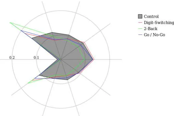
The inter-relations between RR, AR, OR and RNG under the four experimental conditions are clarified by Figure 1, which shows the relative frequency of each type of bigram – repeats, rotations one step clockwise, two steps clockwise, etc. – under the four conditions. The figure illustrates that in the baseline condition there is a general clockwise bias, superimposed upon a bias to adjacent and opposite responses. These biases are magnified in the dual-task conditions, with an increased tendency to adjacent responses coupled with a decreased tendency to repeat responses.
The final statistic, the turning point index (TPI), reflects the tendency to switch between clockwise and counter-clockwise selection on the display. Its value is scaled so that it is 1.0 for an unbiased sequence, with higher values reflecting more frequent switching than chance and low values reflecting a tendency to persist in one direction longer than expected. Under baseline conditions subjects exhibited this tendency (to persist in one direction) – a tendency that was exacerbated under dual-task conditions (with the demanding memory task again having the greatest effect).
The dataset is suggestive of several features of the processes underlying random generation:
a) In order to achieve lower R scores than chance, subjects must either adopt a strategy that ensures good equality of response usage as a side effect (e.g., cycling through responses), or maintain some record of their responses that allows them to avoid choosing any one response too often. There is no evidence to suggest the former.2
chance, even from this unlikely position, of producing the critical item (“A”) on the last response. Thus the probability of generating exactly 10 instances of each response is low. The expected value of R decreases to zero as sequence length increases to infinity.
2
Assuming the latter, this record appears to be compromised (or ignored) in two of the dual-task conditions (resulting, paradoxically, in R scores closer to that expected by chance);
b) The bigram data suggest an underlying bias towards adjacent and opposite responses but away from repeat responses. This bias is magnified in dual task conditions, particularly when the secondary task is the 2-back task; and
c) These two features dissociate, with R resorting to its expected value for two of the secondary task conditions, but bigram statistics being most severely distorted by just one of those conditions.
These features are at least superficially consistent with other studies that suggest dissociable processes underlie random generation, such as those of Towse and Valentine (1997) and Miyake et al. (2000) described above.
3
A Model of Random Generation
The account of random generation offered by Baddeley (1996) and described above is limited in two ways. First, it is specified verbally and therefore open to (mis-)interpretation. Second, it is not specified in the terms of the functional components required to fully operationalise the model. This section presents a process model of random generation based on the verbal account that is a) computationally fully specified, and b) anchored in a more general view of the functional organization of mind.
3.1 Theoretical Background
[image:10.595.191.495.81.284.2]The steps of Baddeley et al.’s account of random generation as described above suggest separable processes for the generation of schema-driven behaviour, the continuous monitoring of behaviour, and the selection or switching of control schemas when appropriate. As noted by Baddeley (1996), such a decomposition of cognitive processing is consistent with the Contention Scheduling / Supervisory System theory of Norman and Shallice (1986; see also Shallice & Burgess, 1996). Within this theory, all behaviour is controlled by schemas
– partially ordered sets of lower-level behaviours. Schema selection is determined by an activation-based competitive process (contention scheduling). This process operates autonomously in routine situations, with schemas receiving excitation or inhibition from an internal model of the environment and from higher level schemas. (See Cooper & Shallice, 2000, for an implementation.) In non-routine situations the operation of contention scheduling is modulated by a second system – the supervisory system – which is held to operate indirectly on behaviour by selectively exciting or inhibiting schema representations within the contention scheduling system.
3.2 Verbal Description of the Model and its Operation
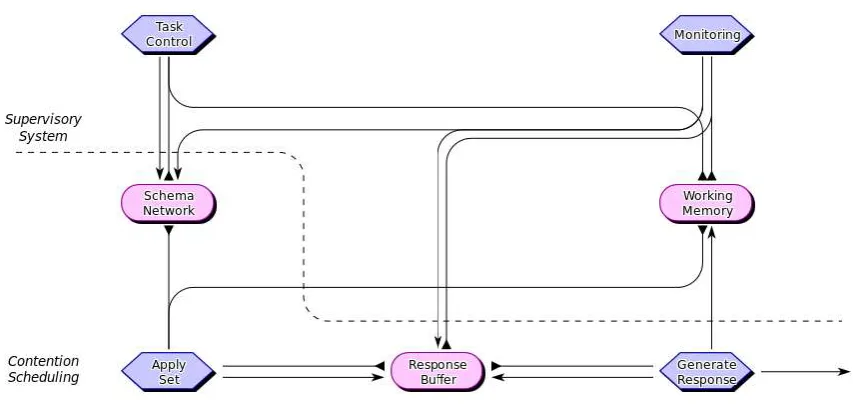
Figure 2 depicts the functional components of the model of random generation.3 The figure adopts a formal graphical language for describing functional decomposition within information processing models in which hexagonal boxes represent processes that transform information, rounded rectangles represent buffers that store information, pointed arrows represent information being sent or written to one component by a process, and flat-ended arrows represent information being read from a buffer by a process (see Cooper & Fox, 1998). All components operate in parallel. The upper portion of the diagram, which operationalises a simplification of the supervisory system, comprises two processes and one buffer. The lower portion, which operationalises the contention scheduling system, comprises two buffers and two processes.
Consider first the components and operation of contention scheduling. Schema Network contains the set of possible schemas that might be used to generate a response, at most of one
3
[image:11.595.78.505.89.292.2]The model and functional architecture presented here is a simplification of a previous model of random generation which was focussed on understanding the effect of rate on random generation performance (Sexton & Cooper, 2014). That model was specified within essentially the same architecture as shown in figure 2. However, the effects of varying the efficacy of the various executive functions were not explored in that model. Equally, that work did not attempt to address dual task interference. Full details of all components of the current model are given in Appendix A. The complete source code (in C) is available at http://www.ccnl.bbk.ac.uk/models/rng_2016.tgz.
of which is active (i.e., controlling behaviour) at any time. Apply Set implements the assumption that successive random responses are produced by the application of the active schema to previous responses. Thus, Apply Set proposes a possible response by consulting Working Memory (for the previously generated item, e.g., “3”) and Schema Network (for the active schema, e.g., “+4”). The putative response (e.g., “7”) is stored in Response Buffer, which is a temporary store that allows a putative response to be vetted before it is actually produced. Production of the response is the job of Generate Response. In paced random generation Generate Response will be triggered by the pacing signal (e.g., a metronome). In self-paced random generation it is assumed that Generate Response normally waits for supervisory processes (specifically Monitoring) to check that a proposed response is sufficiently random before outputting it. On production of a response, Generate Response also copies the response to Working Memory, a component of the supervisory system that stores recent responses and is used both to provide a seed for Apply Set and to ensure (via Monitoring) that successive responses are sufficiently random.
The active schema in Schema Network is set by Task Control, a supervisory system process that is invoked automatically when there is no active schema within Schema Network. This may occur if the active schema decays through inadequate maintenance, or if Monitoring rejects the current schema. Monitoring is a supervisory process that examines a putative response (as stored in Response Buffer), decides if it is sufficiently random (given the history of recent responses stored in Working Memory) and, if not, inhibits production of the response (by clearing Response Buffer) and switches the current schema (by deactivating the active schema in Schema Network).
The main work of the model is done by the two supervisory processes. Monitoring must decide, based on the contents of Working Memory and Response Buffer whether a candidate response is sufficiently random. Working Memory includes a (possibly imperfect) record of recently generated responses, while Response Buffer contains the candidate for the next response. Conceivably there are individual differences in what subjects consider to be “sufficiently random”, but we assume a minimal condition, namely that the candidate response is not a recent response (i.e., is not in Working Memory). Task Control, on the other hand, must propose a schema when none is available. As a working hypothesis, we assume that Task Control involves selecting at random from the available schemas, subject to biases imposed by the response modality. Thus, if responses are numbers given verbally, then Task Control will show a bias towards selecting schemas such as +1 or –1, and away from, e.g., +7. In contrast, if responses are given by selecting from a clock-face display, as in the experiments of Cooper et al. (2012), then Task Control will show a bias towards adjacent and opposite schemas, and away from schemas which select, say, three positions clockwise from the previous response.
As noted earlier, the empirical data indicate that response-modality-induced biases in schema selection are more pronounced under fast paced conditions (Baddeley, 1966; Towse, 1998), when TMS is applied over left DLPFC (Jahanshahi et al., 1998) and under dual-task conditions (Cooper et al., 2012). Given this, we assume that each schema Si has a weight wi,
and the probability of selection of schema Si is given by the Boltzmann equation:
𝑝(𝑆𝑖) = 𝑒 𝑤𝑖⁄𝜏
∑ 𝑒𝑗 𝑤𝑗⁄𝜏 (3)
cognitive resources and varies with task conditions. Full details of the specific schemas and schema weights assumed in the simulations reported here are given in Appendix B.
One further requirement of Task Control is that it should frequently switch the schema guiding the proposal of responses, regardless of whether Monitoring considers a putative response to be insufficiently random. Whatever schema is active, generating a sequence of responses with that schema will ensure that the responses are not random. To avoid this, Task Control periodically deactivates the active schema. Given the processes already described, an alternative schema will then be activated (with the alternative being chosen according to equation 3).
3.3 Parameters of the Model and their Putative Relation to Executive Functions
In addition to the weights of each schema, the model has five key parameters. First, responses are recorded in Working Memory, but it is assumed that decay operates on the contents of Working Memory. Second, recording of responses in Working Memory may be prone to failure. These lead to two distinct parameters: WM Decay Time (the maximum number of processing cycles an element can remain in Working Memory, with probabilistic deletion prior to this) and WM Update Efficiency (the probability that updating is successful). Third, according to the competence model, when a putative response is placed in Response Buffer it is checked by Monitoring to ensure that it is sufficiently random (subject to the model’s conception of randomness). Again, at the performance level it is conceivable that this process does not operate on every putative response, and this leads to a third parameter: Monitoring Efficiency (the probability that monitoring rules are invoked). Finally, two parameters govern the operation of Task Control: Switch Rate (the probability of switching schemas after each response), and Temperature (the value of in equation 3).
The approach to parameterisation aims to clarify potential sources of variation within the model. This results in many, rather than few, parameters. While it might be possible to consolidate some parameters by linking them (e.g., through a single efficiency parameter), this would fail to acknowledge the functional modularity assumed within the underlying architecture and artificially constrain the resultant model. Our approach is rather to be over-zealous, if anything, in the identification of parameters, but to guard against overfitting by then consider the effects (including interaction effects) of variation of each parameter, to fix parameters where they do not affect the model’s behaviour (e.g., because variation in one parameter can be countered by variation of another parameter), and to compare the behaviour of the fully parameterised model with that of restricted versions (e.g., in which parameters are set to optimal values or where parameters are linked). Supporting simulations demonstrating the effects of varying individual parameters are reported in the Supplementary Materials.
4
Simulation 1: The Generation of Random Response Sequences
The purpose of simulation 1 was to demonstrate that, with appropriate parameter settings, the model is able to capture the general patterns in performance observed in human subjects on a random generation task (i.e., the ballpark values for a range of measures of randomness). The target data were those from the baseline condition of experiment 1 of Cooper et al. (2012), as described above. These data were used as a target because a) in contrast to many studies (e.g., those of Baddeley et al., 1998 or Miyake et al., 2000) they include multiple dependent measures and b) the raw data are openly accessible4, allowing additional analyses to be performed for the current work and supporting further analysis by researchers not involved in the original research.
4
4.1 Method
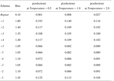
Preliminary simulations with the model revealed that human-like behaviour appeared to occur when:
a) WM Decay Time was approximately 15;
b) schema selection was biased to favour adjacent and opposite responses over other responses, and clockwise responses over count-clockwise responses;
c) schema biases were modulated on a subject-by-subject basis by a moderate level of noise to account for individual differences in those biases (see Appendix B for further discussion of schema biases, schema bias noise, and the precise values of the biases for each schema); and
d) other parameters (WM Update Efficiency, Monitoring Efficiency and Switch Rate) were set to maximal values (1.00 in each case).
Additional simulation work found that the effect of increasing WM Decay Time on each of the dependent measures discussed above (R, RNG, RR, AR, OR and TPI) could be countered by decreasing Monitoring Efficiency. In order to avoid artefacts due to bounds on parameters the simulations reported in this section therefore assume WM Decay Time of 30 and Monitoring Efficiency of 0.65. τ was fixed at 1.00 and weights for each schema were set by hand to generate sequences that appeared, with the naked eye, to yield values of randomness similar to those observed by Cooper et al. (2012). Thirty-six sequences each of 100 simulated responses, corresponding to thirty-six virtual subjects, were then generated by the model. (Note that at this stage no formal method was used to maximise the fit of the model to the human data.) Each simulated sequence was scored on the measures described above, namely R, RNG, RR, AR, OR and TPI.
For comparison, thirty-six pseudo-random sequences of 100 responses were also generated using an unbiased random number generator and scored in the same way in order to estimate chance values (and standard deviations) of the various measures. The procedure therefore yielded three groups of comparable scores, with each derived from 36 (real or virtual) subjects, corresponding to measures of randomness for: the human subject data of Cooper et al. (2012); chance sequences of the same length; and simulated sequences of the same length.
4.2 Results
Means and standard deviations of all dependent measures for the three groups – human subjects of Cooper et al. (2012), chance, and the simulated subjects – are shown in table 2. Inspection of the data suggests that the human data show biases on most if not all measures in comparison to chance. These biases appear to be replicated in the sequences produced by the model. Pairwise between-subjects t-tests revealed that for all dependent measures and in all but one case: a) baseline subject values differed significantly from chance values; b) simulated values differed significantly from chance values; but c) baseline values and simulated values did not differ (see table 3). The one exception was the case of OR (Opposite Responses), where the difference between baseline subject and chance values was sizable but did not quite reach significance (p = 0.059).
4.3 Discussion
Consider first R, equality of response usage. The chance value on this measure (1.840) reflects the fact that in a sequence of 100 independent responses chosen from a response set of 10 it is likely that not all responses are selected exactly 10 times. (If they were, R would be zero.) Human subjects consistently score below the chance value on this measure, indicating (perhaps counter-intuitively) that they produce responses with frequencies that are more equal than would be expected by chance in a 100 item sequence. This suggests not merely that human responses are not independent, but that response selection is somehow biased to actively avoid over-sampling of any particular response. This in turn requires either a strategy with a side-effect of equating response usage (e.g., cycling from one response to the next) or some memory of previous responses (or at least of response frequencies).
Consider now the various bigram biases. In order to achieve human-like values of RR, OR, AR and TPI within the model, the probability of Task Control selecting the “repeat” schema was set to 0.008, while for selecting an “opposite” schema it was 0.164, the probability of selecting the “adjacent clockwise” schema was set to 0.140 and for the “adjacent counter-clockwise” schema it was 0.113. (One might assume chance to be 0.100 for each schema.) While these values were set by hand to produce a good fit to the data, as noted above it is assumed that the values of the dependent measures arising from the human data reflect biases induced by the specific procedure or apparatus. Thus, the clock-face type display from which responses were selected appears to encourage high rates of selection of opposite and adjacent associates, just as two-handed keyboard response collection facilitates alternation in responses between hands. Departing from equi-probable schema selection within the model in order to address response bigram biases is therefore justified.
[image:15.595.74.521.114.318.2]At the same time, if between-subject noise is not introduced into schema biases, the above-quoted settings for biases yield a value of RNG that is substantially lower than observed in human subject group data. To understand why consider two subjects, one with a tendency to favour production of adjacent responses and the other with a tendency to favour production of opposite responses. The first will yield a high score on AR and a low score on OR, while the second will yield the opposite pattern. Both subjects will however score similarly high on the RNG measure. The mean across subjects for AR or OR will therefore be moderate, while for RNG it will be high. It is therefore critical when considering group
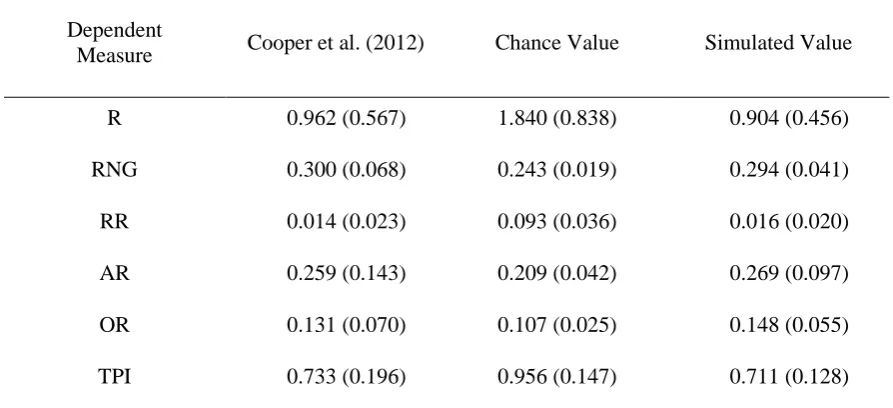
Table 2: Means (and standard deviations) of the six dependent measures for the subject data of Cooper et al. (2012), chance, and simulation results.
Dependent
Measure Cooper et al. (2012) Chance Value Simulated Value
R 0.962 (0.567) 1.840 (0.838) 0.904 (0.456)
RNG 0.300 (0.068) 0.243 (0.019) 0.294 (0.041)
RR 0.014 (0.023) 0.093 (0.036) 0.016 (0.020)
AR 0.259 (0.143) 0.209 (0.042) 0.269 (0.097)
OR 0.131 (0.070) 0.107 (0.025) 0.148 (0.055)
random generation data to consider (and as in the case here, model) individual differences – some group measures of randomness may obscure critical features of individual behaviour (cf. Sexton & Cooper, 2014).
The repeat response (RR) measure is somewhat different from the other bigram measures. Both real and simulated subjects tend to avoid repeats, resulting in a significantly lower value for this measure than would be expected by chance. Towse (1998; see also Towse et al., 2016) suggests that this may be a result of automatically inhibiting a response once it has been generated, as in the Competitive Queueing mechanism of sequential control introduced by Houghton (1990). The model presented here instead assumes that low rates of repeat responses are the result of active monitoring and subsequent inhibition of responses that, according to an individual subject’s conception of randomness, are insufficiently random. Thus repeat responses are proposed (albeit at low rates) by the Apply Set process but then suppressed by Monitoring prior to production by the Generate Response process. The rationale for this is discussed further below in the General Discussion.
The final measure, the turning point index (TPI) is again lower than chance in both real and simulated subjects. This reflects a tendency to favour one direction (clockwise) over the other. Again this reflects properties of the apparatus for response collection (i.e., the clock-face display), but again it is directly addressed within the model by assuming larger schema biases for clockwise selection than for equivalent counter-clockwise selection (e.g., as noted above, the adjacent clockwise schema has bias 0.140, while the adjacent counter-clockwise schema has bias 0.113).
[image:16.595.73.520.111.318.2]Before turning to further empirical support for the model it is instructive to consider the extent to which the model can account for the five “robust behavioural effects” enumerated in the introduction. Most clearly, modality induced response biases (effect 2) may be attributed within the model to the set of available schemas, and their weights, which determine responses. Thus, if one were modelling random generation behaviour as reflected by responses from a two-handed key pad, one would assume that schemas for alternation would be available and strongly weighted. The effect of external representation of the response set (effect 1) may be due to similar factors, as the format of the external representation will likely impose variable schema-selection biases and thereby encourage stereotypy. This may also be the case for the effect of response set size (effect 4), where
Table 3: Pair-wise comparisons between the three datasets of table 2, with t-values (d.f. = 70 in all cases), and two-tailed probabilities.
Dependent Measure
Cooper et al. (2012)
versus
Chance Value
Simulated Value
versus
Chance Value
Cooper et al. (2012)
versus
Simulated Value
R t(70) = 5.203, p < 0.001 t(70) = 5.886, p < 0.001 t(70) = 0.482, p = 0.631
RNG t(70) = 4.925, p < 0.001 t(70) = 6.828, p < 0.001 t(70) = 0.526, p = 0.601
RR t(70) = 11.097, p < 0.001 t(70) = 11.261, p < 0.001 t(70) = 0.426, p = 0.671
AR t(70) = 2.018, p = 0.047 t(70) = 3.421, p = 0.001 t(70) = 0.357, p = 0.722
OR t(70) = 1.920, p = 0.059 t(70) = 4.074, p < 0.001 t(70) = 1.139, p = 0.258
larger response sets will require more schemas for generating a response from earlier behaviour if the full response set is to be produced (and so underlying biases are likely to be more pronounced). The relative lack of repeat responses (effect 3) arises in the model not due to inhibition of immediate responses (which must be overcome to produce a repeat), but due to a combination of a low rate of proposal of repeat responses together with deliberate suppression of repeats, with the latter being compromised when working memory is limited or monitoring for sufficient randomness is impaired. Finally, the effect of response rate (effect 5, with increased rate resulting in increased stereotypy) is a natural consequence of the combination of schema-generated behaviour and the monitoring / checking process. If the latter is compromised due to time pressure then responses will necessarily be more stereotyped.
5
Simulation 2: Experiment 1 of Cooper et al. (2012)
The target data for simulation 1 was from the control or baseline condition of the random generation study of Cooper et al. (2012). Simulation 2 explores whether the model can account for the random generation behaviour observed in the three different secondary task conditions of that study. We show that a) with appropriate values of key parameters the model can account for the behaviour of subjects in the different experimental conditions, but that b) the model is less able to capture artificial datasets, thus demonstrating that the model’s parameters do limit or constrain its observable behaviours. Furthermore, we show that c) reduced forms of the model, with fewer parameters provide statistically less adequate accounts of the data. We interpret the effects of concurrent performance of the different secondary tasks on primary task performance in terms of the required parameter values in each condition. This allows us to infer how different secondary tasks compromise the various processes involved in random generation.
The logic of this simulation study assumes that the values of the various parameters generally reflect the efficacy of different cognitive processes. For example, it is assumed that concurrent performance of a secondary task will reduce the rate of switching between schemas (i.e., Switch Rate will be less than 1.00). Similarly it may reduce the efficiency of the monitoring process, such that it is applied on fewer trials than otherwise (i.e., Monitoring Efficiency may be less than 0.65), or reduce the temperature of the selection processes, such that schema selection is more biased (i.e., Temperature may be less than 1.00).
5.1 A 3-Parameter Model
5.1.1 Method
Given that our aim was to determine parameter values yielding the best fit of the model to different data sets, a brute force approach was taken whereby the reduced model’s output at each point in a 3 dimensional grid of parameter space was scored for the six dependent variables considered in the original empirical work. To ensure good estimates of the model’s behaviour across the parameter space 360 sequences, each of 100 items, were generated at each point in the grid, corresponding to 360 virtual subjects, and mean values of each dependent measure were calculated and recorded for each point, yielding the DV “profile” for that point. The grid itself was defined by Temperature ranging from 0.00 to 2.00, Switch Rate ranging from 0.00 to 1.00, and Monitoring Efficiency ranging from 0.00 to 1.00, each in increments of 0.01. It thus comprised a total of 201 101 101 = 2,050,401 points.
The fitting procedure minimised the difference between observed and simulated behaviour on all six dependent measures simultaneously. Thus, for each of the baseline and three experimental conditions, the fit between model DV profile and subject DV profile was calculated at each point in parameter space as the maximum, over the six dependent measures, of the absolute value of the difference in z scores between the model’s behaviour (based on 360 virtual subjects) and the subject behaviour on that condition. The values of the parameters for which this measure was minimised were taken as the best fitting values for that condition.
In order to determine whether the model was limited in the behaviours that it could produce, best fits were also calculated for two kinds of “artificial” profiles: a) the profile generated by a true random generation process (as given in the Expected Value column of table 1), and b) profiles generated by randomly crossing the actual profiles from the different experimental conditions. The former allows one to evaluate whether the model can fit a true random sequence while the latter allows one to evaluate whether the model can fit an arbitrary DV profile where all values in the profile are within the observed ranges.
5.1.2 Results
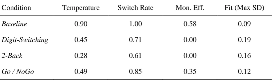
[image:18.595.77.520.108.238.2]Best fitting parameter values and resultant fits for the baseline and three experimental conditions of Cooper et al. (2012) are shown in table 4. Thus, for the baseline condition the best fit (with all six dependent measures lying within 0.09 of a standard deviation of their observed values) was obtained with Temperature = 0.90, Switch Rate = 1.00, and Monitoring Efficiency = 0.58. These values compare favourably with those chosen by hand for simulation 1 (1.00, 1.00, 0.65, respectively), but also demonstrate that the good fit to baseline behaviour presented in that simulation is not the result of cherry-picking parameter values. In fact good fits to the baseline behaviour (within 0.20 standard deviations on all six dependent measures)
Table 4: Best-fitting values of the three parameters and the resultant fits for the baseline and three dual-task conditions of Cooper et al. (2012).
Condition Temperature Switch Rate Mon. Eff. Fit (Max SD)
Baseline 0.90 1.00 0.58 0.09
Digit-Switching 0.45 0.71 0.00 0.19
2-Back 0.28 0.61 0.00 0.16
are obtained with any value of Temperature in the range [0.90, 1.00] and any value of Monitoring Efficiency in the range [0.55, 0.65].
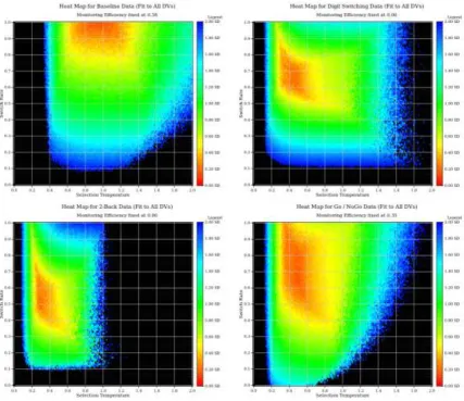
Figure 3 shows heat-maps for cross-sections through the parameter space for each of the four conditions, with Monitoring Efficiency fixed in each case at the values given in table 4. In all four cases a good fit is obtained within a contiguous region of parameter space. The best fitting parameter values reported in table 4 should therefore be viewed as approximate estimates of the relevant parameters under the various conditions. Note in particular that while the best fit for the Digit-Switching condition occurs when Switch Rate is 0.71 (well above the best-fitting value of 0.61 for the 2-Back condition), a good fit is also obtained for this condition with lower values of Switch Rate (e.g., when Switch Rate is 0.61, the measure of fit increases only slightly to 0.21).
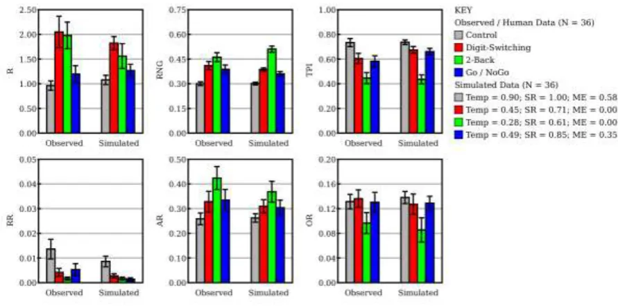
[image:19.595.79.507.71.440.2]The graphs in figure 4 show the observed values of the six dependent variables for each condition along with their values for the best-fitting simulation for each condition. As can be seen from the figure, the best-fitting simulations capture all qualitative effects. Thus, R is highly elevated in the Digit-Switching and 2-Back simulation in comparison to the Baseline simulation, but only slightly elevated in the Go / NoGo simulation in comparison to the Baseline simulation. In contrast, RNG is more highly elevated in the 2-Back simulation (in comparison to the Baseline simulation) than in the Digit-Switching and Go / NoGo simulations, where it is moderately elevated.
With regard to the attempts to fit artificial profiles, the best fit to the true random profile was 2.03 (with Temperature = 1.97, Switch Rate = 0.99, and Monitoring Efficiency = 0.34). That is, the best fit of the model to a true random profile was more than two standard deviations away from the target data on at least one dependent measure. Note though that better fits occur when Temperature is higher, and the model’s performance approaches true chance as Temperature increases to infinity when Switch Rate is 1.00 and Monitoring Efficiency is 0.00. Attempting to fit the model to the crossed profiles revealed that the majority of such profiles (68% of 5000) could not be fit by the model to within 0.20 of a standard deviation. Thus for artificial profiles the best fits were generally poorer (and often substantially so) than for each of the empirically observed profiles, indicating the model is better able to fit human-generated than artificial profiles.
5.2 Model Comparison: Restricted Models
When WM Update Efficiency is held at its maximum value (of 1.0) and WM Decay Time is fixed at 30, as in the above simulations, the model effectively has 3 parameters and is being evaluated for a fit across the four conditions. While the obtained fits (in terms of maximum z scores across the six dependent measures) are held to be good, it is possible that the goodness of fit is largely a result of the number of parameters. Models with fewer parameters might provide statistically better fits. This issue may be addressed by comparing the fit of the 3-parameter model with the fits of 8 reduced models (i.e., 8 models with fewer 3-parameters) using a measure of fit that penalises parameters whose inclusion does not provide a sufficiency improvement in fit. The Bayesian Information Criterion is one such measure.
5.2.1 Method
Eight reduced models were constructed from the full 3-parameter model by restricting parameters as follows:
Model 2: Temperature fixed at 1.0
Model 3: Switch Rate fixed at 1.0
Model 4: Monitoring Efficiency fixed at 0.6
[image:20.595.73.519.84.305.2] Model 5: Switch Rate = Monitoring Efficiency
Model 6: Temperature fixed at 1.0 and
Model 7: Temperature fixed at 1.0 and Monitoring Efficiency fixed at 0.6
Model 8: Monitoring Efficiency fixed at 0.6 and Switch Rate fixed at 1.0
Model 9: Temperature fixed at 1.0 and Switch Rate = Monitoring Efficiency
Models 2, 3 and 4 explore whether each of the three remaining parameters is necessary. Each of these models eliminates one effective parameter by holding it fixed at a value that, from simulation 1, is known to yield a near maximal fit for the baseline condition. Model 5, in contrast, explores the possibility that a single efficiency parameter, specifying both Switch Rate and Monitoring Efficiency, might be sufficient to account for the data. These four models (models 2, 3, 4 and 5) thus have 2 effective parameters. Models 6 to 9 combine the constraints in models 2 to 5, and have just one effective parameter.
For each of the nine models, the Bayesian Information Criterion was calculated using equation 4:
𝐵𝐼𝐶 = 𝑛 + 𝑛 ∙ ln 2𝜋 + 𝑛 ∙ ln𝑆𝑆𝐸
𝑛 + (𝑘 + 1) ∙ ln 𝑛 (4)
where n is the number of conditions, SSE is the minimum sum squared error between the model and the data across the four conditions, and k is the number of parameters in the model. SSE was calculated as the sum of squares of fits over the four conditions, where the fit for each condition was calculated as the minimum of the maximum z-score difference across the six dependent measures between the observed data and the simulated data (i.e., using figures as in table 4).
5.2.2 Results
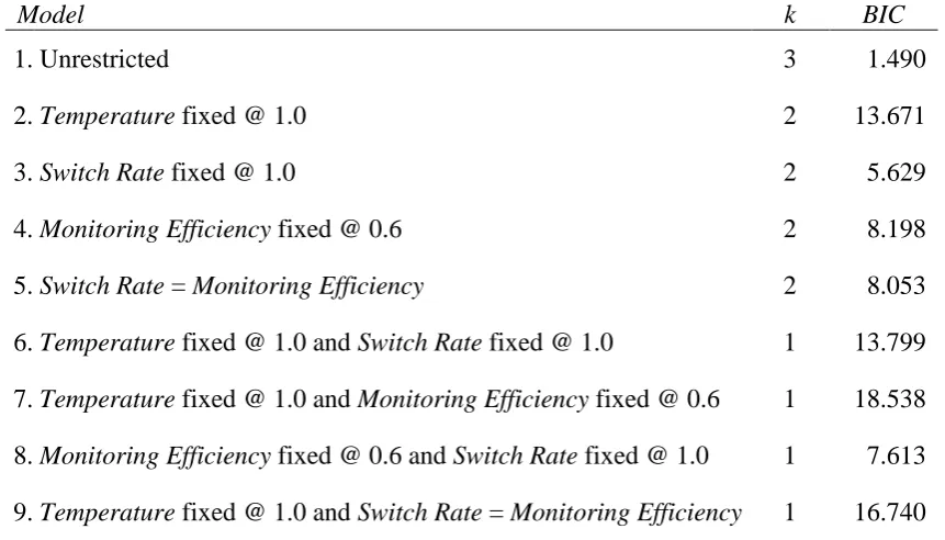
[image:21.595.84.515.110.356.2]Table 5 shows the number of parameters and BIC scores for each of the nine models. Model 1 is preferred on the grounds that, despite having more parameters than the other models, its BIC score is substantially lower than that of any other model. In other words, the extra degrees of freedom of model 1 given by the additional parameters in comparison to the other models is more than compensated for by the improvement in fit of model 1 in comparison to
Table 5: The nine models, the number of parameters (k) in each model, and their Bayesian Information Criterion (BIC) scores.
Model k BIC
1. Unrestricted 3 1.490
2. Temperature fixed @ 1.0 2 13.671
3. Switch Rate fixed @ 1.0 2 5.629
4. Monitoring Efficiency fixed @ 0.6 2 8.198
5. Switch Rate = Monitoring Efficiency 2 8.053
6. Temperature fixed @ 1.0 and Switch Rate fixed @ 1.0 1 13.799
7. Temperature fixed @ 1.0 and Monitoring Efficiency fixed @ 0.6 1 18.538
8. Monitoring Efficiency fixed @ 0.6 and Switch Rate fixed @ 1.0 1 7.613
the other models. It is also of note that the models in which Temperature is fixed (models 2, 6, 7 and 9) perform very poorly (all with BIC scores above 13). Moreover models in which Monitoring Efficiency is fixed perform more poorly than equivalent models in which Switch Rate fixed (i.e., model 4 versus model 3, model 7 versus 6). This suggests that a) variation in Temperature is more critical than variation in any other parameter for capturing the behavioural data, while b) variation in Switch Rate is less critical than variation in any other parameter for capturing the behavioural data.
5.3 Discussion
When allowed to vary the three key parameters of Temperature, Switch Rate, and Monitoring Efficiency arbitrarily, the model can provide a good fit to human random generation behaviour in all four conditions of Cooper et al.’s (2012) study. This may seem unsurprising given the number of parameters that have been varied, but given that fitting each condition requires simultaneously fitting the values of six dependent measures it is not a straightforward result. The facts that the model is also generally less able to fit various “artificial” profiles, and that reduced forms of the model with fewer parameters provide statistically poorer fits to the behavioural data, add further weight to this claim.
Modelling of secondary task interference suggests that the effect of a secondary task is not just to magnify inherent schema selection biases (modelled by a reduction in Temperature), but also to reduce both the rate of schema switching and the efficiency of monitoring processes (or equivalently, the persistence of items in working memory). The three secondary tasks of Cooper et al. (2012) differ in the impact that their concurrent performance has on each of these mechanisms. Thus, the Go / NoGo task is least disruptive, being well-modelled by a relatively moderate reduction in Temperature (from 1.00 to 0.49), a relatively small reduction in Switch Rate (from 1.00 to 0.85), and a sizable reduction in Monitoring Efficiency (from 0.65 to 0.35). Further reductions in each of the three parameters allows the effect of concurrent performance of the Digit-Switching task on random generation to be captured, though the additional reduction in Temperature is small (down to 0.45) and arguably unreliable, in comparison to the reduction in the other two parameters (down to 0.71 and 0.00, respectively). That the best fit is obtained with Monitoring Efficiency at 0.00 is considered below, though this is also found for the 2-Back condition, which in addition requires a further substantial reduction in Temperature (down to 0.28) together with a further small reduction in Switch Rate (down to 0.61).
How should these results be interpreted? One possibility is that the three tasks vary on a single dimension, such as difficulty, with the 2-Back task being hardest and hence having greatest effect on all three parameters (and with Monitoring Efficiency subject to a floor effect) and the Go / NoGo task being easiest and hence having least effect on all three parameters. The model supports a more nuanced account, however. First, all three secondary tasks appear to compromise monitoring of the primary task, though less so for the Go / NoGo task.5 This is evidenced both by the best fitting parameters values across conditions from the full 3-parameter model and by the relatively poor fits of reduced models in which Monitoring Efficiency was fixed. Together, this evidence supports the idea of a separable monitoring process that, under dual-task conditions, must be shared by multiple tasks. Second, set-shifting or switching is compromised in all dual task conditions. Again, this is evidenced both by the best fitting parameter values in the 3-parameter model and by the relatively poor fits of
5
reduced models in which Switching was fixed. That switching might be compromised in dual task conditions is plausible if only because when dual-tasking one must frequently switch between the primary and secondary tasks. Third, the choice of which schema to switch to is also affected in all dual task conditions – models in which the Temperature parameter is fixed at a value that yields a good fit in the baseline condition perform poorly when evaluated across the full dataset – though this choice appears to be particularly compromised when simultaneously performing the 2-Back task.
Note that this account does not make explicit appeal to a ‘response inhibition’ executive function. The original empirical work assumed that the Go / NoGo task would (primarily) tap this function, based in part on the theoretical perspective of Miyake et al. (2000). There is mounting evidence to question whether response inhibition is in fact a distinct executive function (e.g., Hampshire & Sharp, 2015; Miyake & Friedman, 2012), and the current model does not include a specific response inhibition function (though inhibition of putative responses does occur when the Monitoring process detects a putative response that is insufficiently random; cf. figure 2).
Monitoring Efficiency concerns rejecting individual responses in the context of (memory of) previous responses. The model accounts for the effect of concurrent performance of a secondary task on random generation by assuming that recent responses are reliably encoded in a short-term store but that (one form of) variation from baseline performance arises through intermittent failure of monitoring of putative responses with reference to this store. When monitoring is completely disabled, random generation reduces to intermittent switching between schema-based responses, with the difference in interference patterns resulting from differences in the rate of switching and the strength of bias in choosing schemas when switching.
With regard to switching, the 2-Back task appears to affect Switch Rate more than the Digit-Switching task, with it being reduced to 0.61 for the best fitting model in the former condition and 0.71 in the latter condition. While this may seem counter-intuitive, it is unclear whether the difference is statistically significant – reasonable fits in both conditions can be obtained with an intermediate value.6 However, it is noteworthy that in the empirical study Digit-Switching required that subjects switch stimulus-response mappings on every four trials, and not on every trial. In other words, the Digit-Switching task was not maximal in its set-shifting requirements. Moreover, while the 2-Back task is normally viewed as a task that draws on working memory monitoring and maintenance, if working memory maintenance is achieved through a rehearsal process, then successful performance in the 2-Back condition may involve frequent shifting between this rehearsal process and the primary task, thus compromising switching within the primary task. To explore the viability of this hypothesis it will be necessary to integrate a complete process model of the 2-Back, and other, secondary tasks with the model of random generation. One consequence of this would be clarification of the extent to which the three secondary tasks are “process pure” (i.e., the extent to which each taps one and only one executive function). Additional empirical work, in which the switching frequency of the Digit-Switching task were varied, would also speak to this hypothesis.
Interpretation of the Temperature parameter, and how it is affected by the different secondary tasks, is more complex, partly because its affects are determined by an equation rather than a complete process account of schema selection biases. The parameter is clearly important, however, as shown by its importance in the model comparison study. We consider the interpretation of Temperature in more detail in the General Discussion.
6 Fixing Switch Rate at 0.66 and Monitoring Efficiency at 0.00 results in a best of 0.22 for the Digit-Switching