Munich Personal RePEc Archive
A Three-Sector Model of Structural
Transformation and Economic
Development
Bah, El-hadj M.
The University of Auckland
November 2007
Online at
https://mpra.ub.uni-muenchen.de/32518/
A Three-Sector Model of Structural
Transformation and Economic
Development
∗
El-hadj M. Bah
†Department of Economics, University of Auckland, Auckland, New Zealand
March, 2010
Differences in total factor productivity (TFP) are the dominant source of the large variation of income across countries. This paper seeks to under-stand which sectors account for the aggregate TFP gap between rich and poor countries. I propose a new approach for estimating sectoral TFP using panel data on sectoral employment shares and GDP per capita. The approach builds a three-sector model of structural transformation and uses it to infer time paths of sectoral TFP consistent with the reallocation of labor between sectors and GDP per capita growth of a set of developing countries over a 40-year period. I find that relative to the US, developing countries are the least productive in agriculture, followed by services and then manufacturing. The findings are consistent with the evidence from micro data and the approach has the novelty to measure sectoral TFPs over the long term.
Keywords: Productivity, Sectoral TFP, Structural Transformation,
Eco-nomic growth, EcoEco-nomic Development
JEL Classification: O14, O41, O47
∗I would like to thank my advisor Dr. Richard Rogerson for his invaluable advice and guidance. I
am grateful to Dr. Berthold Herrendorf, Dr. Josef C. Brada and Dr. Edward C. Prescott for their advice. I have also benefited from comments by the seminar participants of the Arizona State University Macro working group.
1. Introduction
Income differences across countries are large: income per capita for the US in 2000
was about 30 times the average for the least developed countries. Growth accounting
exercises point to differences in total factor productivity (TFP) as the biggest source of
cross-country income differences1. In this paper, I ask which economic sectors account
for this TFP gap. The answer to this question is important for two reasons. First, it can
help us construct theories for explaining the low productivity in developing countries.
Second, it can be useful for formulating policy recommendations.
The key challenge for measuring sectoral TFP in developing countries is data
availabil-ity. A simple sectoral growth accounting exercise requires comparable data for sectoral
value added in constant prices, sectoral capital stock and sectoral employment. Only
data for sectoral employment is available for developing countries. This data limitation
has led researchers to use indirect methods for estimating sectoral TFPs. The existing
literature uses data on cross-section prices in a multi-sector growth model to infer sectoral
relative TFPs2.
A key contribution of this paper is to show how data on structural transformation, i.e.,
the reallocation of labor across sectors as an economy develops, can be used to uncover
sectoral TFP differences. Kuznets included the process of structural transformation as
one of six stylized facts of economic development. He found that developed countries all
followed a similar process. However, as Bah (2009) documents, many developing countries
are following processes that are very different from the path of developed countries.
It is then natural to think that cross-country differences in the process of structural
transformation provide information about cross-country differences in aggregate income
and productivity.
Specifically, I extend the neoclassical growth model to include three sectors
(agricul-ture, manufacturing and services) and use it to infer sectoral TFP time series consistent
with GDP per capita growth and structural transformation over a 40-year period.
Follow-1
Examples include Hall and Jones (1999), Prescott (1998), Klenow and Rodriguez-Clare (1997), Parente and Prescott (1994, 2000), Hendricks (2002), Caselli (2005).
2
ing Rogerson (2008), the model incorporates two channels that drive labor reallocation
between the sectors associated with structural transformation: income and substitution
effects. First, non-homothetic preferences through a subsistence requirement drive labor
out of agriculture3. Second, a TFP growth differential and the elasticity of substitution
between the manufacturing and service sectors drive the reallocation of labor between
those two sectors4.
I calibrate the model to match the structural transformation and per capita GDP
growth for the US over the period 1950-2000. I then use the calibrated model to infer time
paths of sectoral TFP that are consistent with the structural transformation and economic
development experiences of three developing countries with very different income levels:
Cameroon, Brazil and Korea5.
In this exercise, I assume that preferences are similar across countries but allow all
sectoral TFPs to vary. I show that given data on sectoral employment and aggregate
GDP per capita, the model can be used to infer the time series for sectoral TFPs. The
actual implementation of the approach is somewhat complex because of the dynamics
associated with capital accumulation, but at a heuristic level, the approach works as
follows. Given the calibrated preference parameters, observed employment in agriculture
determines the level of agricultural TFP. Relative employment in manufacturing and
services determines the relative TFPs of those two sectors. Finally, aggregate GDP per
capita determines the levels of TFP in manufacturing and services.
Using this approach, I find that relative to the US, developing countries are the least
productive in agriculture, followed by services and then manufacturing. Korea had high
TFP growth in all three sectors and it was catching up to the US during the 40-year
period. Relative to the US, Cameroon and Brazil did not improve their productivities in
agriculture and fell behind in services. In manufacturing, Cameroon lost ground to the US
while Brazil experienced a modest catch-up especially between 1960 and 1980. I also use
my inferred aggregate capital stock from the model to conduct a simple growth accounting
3
Authors using this feature include: Echevarria (1997), Kongsamut et al. (2001), Laitner (2000), and Gollin et al. (2002, 2007).
4
This feature is used by Beaumol (1967); Ngai and Pissarides (2007). 5
exercise for Korea. I find, similarly to the literature (e.g (Young, 1995), (Bosworth and
Collins, 1996)), that capital accumulation played the primary role, followed by TFP and
labor6.
My findings on relative sectoral productivity are consistent with the available evidence
from micro and producer data. The finding that developing countries are the least
pro-ductive in agriculture is not new. It is a robust finding of the development literature that
compares productivity of agriculture and non-agriculture7. There is also a vast
litera-ture that estimates agricultural production functions across countries and try to find the
determinants of low productivity for developing countries8.
Between manufacturing and services, the micro data collected by the McKinsey Global
Institute and analyzed by Bailey and Solow (2001) and Baily et al. (2005) show that
relative to the US, developed and developing countries are less productive in services
than in manufacturing. This sectoral ranking holds for both labor productivity and TFP.
For instance, Baily et al. (2005) finds that while Turkey’s labor productivity is at 66%
of the US in manufacturing, it is only at 33% in services. Duarte and Restuccia (2010)
used a similar three-sector model to examine sectoral labor productivity for a group
of developed and developing countries. They also find that relative to the US other
countries are the least productive in agriculture and services. In contrast, Herrendorf
and Valentinyi (2007) uses cross-section relative prices from expenditure data from the
Penn World Table (PWT) and finds that relative TFP differences in services are small
compared to consumption goods, construction and equipment goods sectors.
This paper is related to the large literature studying income differences across
coun-tries. Closely related, are a number of papers that focus on the sectoral composition of
output to study aggregate outcomes9. A number of papers emphasize the role of
struc-tural transformation in the development and growth experiences of countries. Gollin et
al. (2002, 2007) show the importance of agriculture in the delaying the start of modern
6
In this exercise, I don’t include human capital which would have the effect of decreasing the role of TFP and increasing that of labor.
7
See Kuznets (1971), Gollin et al. (2002, 2007), Young (2008), Restuccia et al. (2008). 8
Examples include Hayami and Ruttan (1970, 1985) and Mundlank (2001). 9
economic growth. Duarte and Restuccia (2010) has a model similar to mine but focuses
on labor productivity to explain growth episodes and disasters in a number of countries.
Hsieh and Klenow (2007) and Herrendorf and Valentinyi (2007) also use general
equi-librium models to infer sectoral TFPs but instead use cross-section price data from the
PWT. Hsieh and Klenow (2007) focuses on sectors producing consumption and
invest-ment goods while Herrendorf and Valentinyi (2007) include services, consumption goods,
construction and equipment goods.
The rest of the paper is organized as follows. Section 2 describes the model and
characterizes the competitive equilibrium. Section 3 calibrates the model to the US
economy. Section 4 applies the model to a sample of developing countries and find their
time paths of sectoral TFP. Section 5 discusses the findings and section 6 concludes.
2. A Three-Sector Model of Structural Transformation
This section develops a three-sector model of structural transformation, which is
char-acterized as follows. Early in the development process, the majority of the labor force
is engaged in food production. As food output rises, labor moves from agriculture into
manufacturing and services. This is the first phase of structural transformation. In the
second phase, labor moves from agriculture and manufacturing into services. This
pro-cess of structural transformation has been followed by current developed countries but as
Bah (2009) documents, many developing countries are following processes that are very
distinct from the above process. The share of services in output is high at relatively low
income per capita in many developing countries in Africa and Latin America. This is not
the case for Asian countries that are mostly following the path of developed countries.
The model developed here will emphasize differential in sectoral productivity growth as
the main feature explaining differences in structural transformation processes. The model
will be calibrated to match the growth and structural transformation of the US economy
for the period 1950-2000. In the next section, the calibrated model will be used to infer
2.1. Model
At each period, the economy has three sectors that produce each one good: agriculture,
manufacturing and services. A key for the model is to replicate the labor reallocation
across different sectors of the economy. Following Rogerson (2008), the model has two
features to achieve this outcome: non-homothetic preferences and technological growth
differential across sectors. If income elasticities are not all unitary, then resources are
reallocated across sectors as the income increases. Examples emphasizing this feature
in-clude Echevarria (1997), Kongsamut et al. (2001), Laitner (2000), and Gollin et al. (2002,
2007). Technological growth differential and non-unitary elasticities of substitution across
goods lead to resource reallocation across sectors. This feature has been emphasized by
Beaumol (1967) and Ngai and Pissarides (2007).
To simplify the analysis, I assume closed economies, which seems reasonable given the
structure of my model 10.
2.1.1. Preferences
There is a representative household who lives forever. For simplicity, I assume the size of
the household is constant. The household supplies labor to the three sectors and uses its
wage compensation to consume three final goods: an agricultural good, a manufactured
good and services. Lifetime utility is given by:
∞
X
t=0
βtU(Φt, At), β ∈(0,1) (1)
Instantaneous utility is defined over the agricultural good (At) and a composite
con-sumption good (Φt) which is derived from the manufacturing and service sectors. The
instantaneous utility is given by:
log(Φt) +V(At) (2)
10
V(At) is non-homothetic and is given by:
V(At) =
−∞ if At< A
min(At, A) if At≥A
(3)
This specification assumes that there is a subsistence levelA below which the household
cannot survive. This feature has been shown to be quantitatively important for driving
labor out of agriculture11. While the specification seems to simplify the analysis of the
model, we will see later that it also describes the data reasonably well.
The composite good is a CES aggregate of the manufactured good (Mt) and services
(St)12.
Φt=λM
ǫ−1 ǫ
t + (1−λ)S
ǫ−1 ǫ
t
ǫ ǫ−1
, ǫ∈(0,1) and λ∈(0,1) (4)
2.1.2. Endowments
In each period the household is endowed with one unit of time, all of which is devoted to
work. Also, the household is endowed with initial capital stock at time 0 and the total
land for the economy. I normalize the size of land to 1 and assume that land does not
depreciate.
2.1.3. Technologies
Agriculture: My specification for agriculture is very basic. The agricultural good is
produced using a Cobb-Douglas production function with labor (N) and land (L) as
the only inputs. This formulation assumes that capital and intermediate inputs are not
used in the production technology. Quantitatively, the effects of capital and the use
of intermediate inputs are implicitly captured by agricultural TFP. Given that different
countries have different intensities in their use of capital and intermediate inputs in
agriculture, the estimated relative TFP may be biased. However, it is unlikely that
11
See Echevarria (1997), Kongsamut et al. (2001), Laitner (2000), and Gollin et al. (2002, 2007) 12
this will overturn the finding that agriculture is relatively the least productive sector in
developing countries which is a very robust finding of the development literature.
The agricultural good is only used for consumption so the resource constraint is given
by:
At =AatNatαL1
−α
t (5)
where the TFP evolves according to: Aat = Aa(1 +γat)t. The TFP parameter Aa and
γat in the equation above are assumed to be country specific. There are many sources
of cross-country differences in agricultural efficiency. One source is government policies
and institutions that have an impact on agricultural activity13. As an example, it has
been shown that marketing boards, present in many African countries until the 1990s,
were inhibiting the development of the agriculture sector14. Another source of variation
is the quality of land available per person and the climate(s) prevailing in the country.
For example, a variety of seed developed for one region will not necessarily be suited for
another.
Manufacturing and Services: The manufacturing and service sectors produce
output using standard Cobb-Douglas production functions with capital and labor as
inputs. I assume identical capital shares in both sectors which is consistent with estimates
by Herrendorf and Valentinyi (2008) for the US economy15. The manufacturing sector’s
output is used for consumption (Mt) in the composite good and investment (Xt). The
manufacturing sector resource constraint is:
Mt+Xt=AmtKmtθ N1
−θ
mt (6)
where TFP evolves as: Amt =Am(1 +γmt)t. The law of motion of the aggregate capital
13
Restuccia et al. (2008) finds that the lack of use of intermediate inputs and distortions in the labor market explain a big part of the large disparity in agricultural productivity between rich and poor countries
14
These are governmental institutions that buy export crops from farmers at fixed low prices, then resell them abroad at world prices. See Sachs and Warner (1995), Wacziarg and Welch (2008) for details. 15
stock (Kt) in the economy is given by:
Kt+1 = (1−δ)Kt+Xt (7)
where δ is the depreciation rate.
The output of the service sector is only used for consumption through the composite
good. Therefore, resource constraint for the service sector is given by:
St=AstKstθN1
−θ
st (8)
where TFP evolves as: Ast =As(1 +γst)t.
In the equations above, the TFP parameters Am, As, γmt and γst are also assumed to
be country specific. Recovering how these differ across countries is the main contribution
of this paper. Again, a country’s institutions and policies affect its productivity in these
economic activities.
2.2. Equilibrium
In this section, I describe how to solve for the competitive equilibrium of the model
economy from the start of structural transformation16. Note that there are no
distor-tions in the economy, therefore the equilibrium allocadistor-tions can be obtained by solving
a social planner’s problem17. Let T be the first period in which the economy can move
labor out of agriculture. From period T on, a social planner chooses the allocations
(Kt, Kmt, Kst, Nat, Nmt, Nst, St, Lt) to solve the following maximization problem:
max ∞
X
t=T
βt−T
(log(Φt) +V(At))
s.t
Φt =λM
ǫ−1 ǫ
t + (1−λ)S
ǫ−1 ǫ
t
ǫ ǫ−1
16
The definition of competitive equilibrium is standard so I do not reproduce it here. 17
A=AatNatαL1
−α
t
St=AstKstθN
1−θ st
Mt+Xt=AmtKmtθ N
1−θ mt
Kt+1 = (1−δ)Kt+Xt
Kmt+Kst =Kt
Nat+Nmt+Nst = 1
In what follows, I develop a solution method similar to that for the one sector growth
model. Recalling that we normalized land to be one, and given the preferences over food
consumption, we can easily solve for employment in agriculture; which depends only on
productivity in the agriculture sector:
Nat =
A Aat
α1
(9)
LetNt= 1−Nat be the total time that can be allocated between the manufacturing and
service sectors. Then the problem is reduced to solving the following two-sector planner’s
problem:
maxP
βt ǫ ǫ−1
loghλ AmtKmtθ N
1−θ
mt + (1−δ)Kt−Kt+1
ǫ−ǫ1
+ (1−λ)A
ǫ−1 ǫ
st K
ǫ−1 ǫ θ
st N
ǫ−1 ǫ (1−θ)
st
i
s.t
Kmt+Kst =Kt (10)
Nmt+Nst =Nt (11)
The F.O.C for this problem are given by:
λAmtKθ
−1
mt N
1−θ mt M
−1
ǫ
t = (1−λ)A
ǫ−1 ǫ
st K
ǫ−1 ǫ θ−1
st N
ǫ−1 ǫ (1−θ)
st (12)
λAmtKmtθ N
−θ
mtM
−1
ǫ
t = (1−λ)A
ǫ−1 ǫ
st K
ǫ−1 ǫ θ
st N
ǫ−1 ǫ (−θ)
M−1ǫ
t−1ϕ
−1
t−1
M−1ǫ
t ϕ
−1
t
=β
"
1−δ+θAmt
Kt
Nt
θ−1#
(14)
where
ϕt=λM
ǫ−1 ǫ
t + (1−λ)S
ǫ−1 ǫ
t (15)
Equations (12) and (13) equate marginal products of capital and labor in manufacturing
and services. Equation (14) states that the marginal rate of intertemporal substitution
of the consumption good equals to the marginal rate of transformation of current
con-sumption to future concon-sumption.
Dividing equation (12) by (13) and combining with (10) and (11), yields:
Kmt
Nmt
= Kst
Nst
= Kt
Nt
(16)
i.e.; capital to labor ratios are equalized across sectors.
Using equation (16) in (12) leads to:
1−λ
λ
Mt
St
1ǫ
= Amt
Ast
(17)
This equation gives the relative consumption of services and the manufactured good.
Note that this ratio depends only on current period productivities. Let Ct be the
non-agricultural aggregate expenditures. I show in the appendix that:
Ct=
ϕtM
1
ǫ
t
λ (18)
where ϕt is as defined in equation (15).
Equations (14) and (18) then imply:
Ct
βCt−1
= 1−δ+θAmt
Kt
Nt
θ−1
(19)
This equation is similar to the standard Euler equation for the one sector growth model
with production function:
F(Kt, Nt) = Amt
Kt
Nt
θ
Nt (20)
Equations (9), (16), (17), (19) and the resource constraint equations (10) and (11)
completely characterize the equilibrium allocations. I show in the appendix that one
can reduce the problem of solving for the equilibrium allocations to a unique dynamic
equation of capital.
Kt+1 = Amt
Kt
Nt
θ
Nt+ (1−δ)Kt−β
"
1−δ+θAmt
Kt
Nt
θ−1#
" Amt−1
Kt−1
Nt−1
θ
Nt−1+ (1−δ)Kt−1−Kt
#
(21)
Given the initial capital stock and transversality condition, we can solve for the path of
aggregate capital stock for the economy using equation (21). Once capital is known, all
other allocations can be easily derived. In particular, I show in the appendix that the
quantity of labor used in the service sector is given by:
Nst =
Ct Amt Kt Nt θ
1 + λ
1−λ
ǫAst
Amt
1−ǫ (22)
where Ct is given by:
Ct=Amt
Kt
Nt
θ
Nt+ (1−δ)Kt−Kt+1 (23)
The strategy for computing the equilibrium allocations can be summarized as follows.
Non-agricultural labor is computed using equation (9). From equation (21), I compute
the path of aggregate capital in the economy. Equation (23) gives the sequence of the
composite consumption good. Finally, from equation (22) I derive the hours in the service
sector. The other series: sectoral capital, labor in manufacturing and sectoral outputs
are then easily derived.
For the equilibrium prices, I normalize the price of the manufactured good to 1 in each
relative to the manufactured good. The wage rate and rental rate of capital are the
marginal products of labor and capital of the manufacturing technology. Given wage
equality between sectors, we have:
pst =
Amt
Ast
(24)
This equation results from the equality of capital share in manufacturing and services
which leads to the same capital to labor ratio across the two sectors. The relative price
of the agricultural good is the wage rate divided by the marginal product of labor in
agriculture18:
pat =
wt
αAatNα
−1
at
(25)
In the next sections, I will compute the transition dynamics of the model. In all
cases, I don’t assume that countries are on a balanced growth path. In the model’s
framework, a balanced growth path exists only when the agricultural sector disappear
and manufacturing TFP grows at a constant rate. Moreover, it can be shown that if in
addition, the elasticity of substitution between manufacturing and services is not unity,
then there is structural transformation along the asymptotic balanced growth path19.
3. Calibration to the US Economy
In this section, I calibrate the model to the US economy for the period 1950-2000. The
sources and detail of the data series are explained in the appendix.
3.1. Parameter Values
The model is calibrated to match the U.S structural transformation and GDP per capita
growth from 1950 to 2000. The model period is 1 year. The natural counterpart for
labor input in the model is sectoral shares of hours worked, this will be used for the
18
There is a long literature on dualism of the labor market in developing countries which the model abstract from.
19
calibration20. The parameter values to determine are A, β, δ, ǫ, λ and the time series for
Aat, Amt, Ast. I assume constant TFP growth rates for manufacturing and services for
the US.
Choosing values for the productivity levelsAi(i=a,m,s)amounts to choosing units;
there-fore, I normalize those to 1 in 1950. I set the labor share in agriculture α to 0.7 to be
consistent with the empirical findings of Hayami and Ruttan (1985) and Mundlank (2001).
The capital share θ is set to 0.33 as estimated by Herrendorf and Valentinyi (2008).
Contrary to the standard calibration method for growth rates, discount factor and
depreciation rate parameters, I don’t assume that the US economy is on a balanced
growth path21. Instead, I calibrate the parameters (γ
m, γs, β, and δ) jointly to match
four averages in the data from 1950 to 2000: average growth rate of GDP per capita,
average growth rate of the price of services relative to manufacturing, average investment
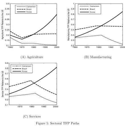
to output ratio and average capital to output ratio. Table 1 shows the targeted statistics
from the model and the data.
The average GDP per capita growth rate is linked to the manufacturing TFP growth
rate. Asymptotically, GDP growth depends only on manufacturing TFP growth. The
average growth rate of the price of services relative to manufacturing will be used to find
the service TFP growth rate. From equation (24), we have:
log(pst) = log(Amt)−log(Ast) (26)
Differentiating this equation with respect to time approximating, yield:
∆ps=γm−γs (27)
where ∆pst is the slope of the price of the service good relative to the manufactured
good. From the Groningen 10-sector industry database, I calculated the relative price of
services from 1950 to 200022. On average, the price of services relative to manufacturing
20
In the next session when applying the model to developing countries, I will use sectoral employment shares because data for sectoral hours is not available for all the countries considered in my sample. 21
In 1950, the share of agriculture in total output was 7.9% and it decreased to 1.16% in 2000. 22
increased by 0.88% per year. Then, γs = γm−0.0088. The last two targeted statistics
will help determine the discount factorβ and depreciation rate δ.
The agricultural productivity growth rate parameterγat and the subsistence levelAare
determined using the agricultural share of hours worked. The growth rate of agricultural
productivity is set so that the model matches the US agricultural shares of hours worked.
I assume that the growth rate varies each decade starting in 195023. The growth rate
between two dates t1 and t2 is calculated as follows:
γat
1t2 =
Nat1
Nat2
t α
2−t1
−1 (28)
where Nat is the agricultural share of hours at date t . The subsistence level is just the
agricultural output in every period after the start of structural transformation. Because
I normalized agricultural TFP to be 1 in 1950, it follows:
A=Naα1950 (29)
Lastly, I need to calibrate the initial capital k0 and the parameters ǫ and λ. The
parameter ǫis the elasticity of substitution between manufacturing and services andλ is
the weight of the manufactured good in the production of the composite good. The initial
capital is chosen to match the share of hours in manufacturing in 1950. The calibrated
value is 2.8. The parameters ǫ and λ determine the labor reallocation between the
manufacturing and service sectors. For labor to be reallocated from the high productive
sector (manufacturing) to the low productive sector (services), ǫhas to be between 0 and
1. In other words, ǫ−1
ǫ has to be negative. I choose values of ǫ and λ to minimize the
quadratic norm of the difference between the predicted and actual manufacturing shares
of hours worked between 1950 and 2000. The corresponding values are: ǫ = 0.45 and
λ = 0.01. While there are no standard values for these two parameters, the estimates
23
by Duarte and Restuccia (2010) are respectively 0.4 and 0.0424. Table 2 summarizes the
calibrated parameter values.
3.2. Structural Transformation of the US economy
This section provides some insights into how well the calibrated model fits the data. I
use the calibrated model to compute the sectoral shares of hours of the US economy from
1950 to 2000 and compare them with the data series25.
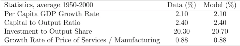
Figure 1 shows the structural transformation predicted by the model. It shows that the
model does a good job at replicating the sectoral shares of hours worked. By construction,
the model matches exactly the agricultural share of hours for the years used in the
calibration. But the model also does a good job in the other years. Of greater interest
is the fact that there is a close match between the model and the data in the other two
sectors. In particular, the model traces very well the shares of hours in the manufacturing
and service sectors until the early 1990s. However, starting from the mid 1990s, the data
show a drop in manufacturing share of hours that is not well replicated by the model.
This discrepancy is caused by two factors.
First, the model abstracts from increases in total hours worked. However, as Rogerson
(2008) shows, there have been a substantial increase in total hours worked in the US
starting from the mid 1980s and most of the increase occurred in the service sector. By
abstracting from growth in total hours and using sectoral shares, the model does not
capture the full increase in the share of services. I abstract from growth in total hours
because such data is not available for the developing countries for which the model will
be used to determine sectoral TFP paths in the next section.
The second issue is the assumption of constant growth rates for productivity in
manu-facturing and services. In fact, Brauer (2006) of the Congressional Budget Office reported
that there was an acceleration of manufacturing productivity since 1979. In my model,
this acceleration would lead to a decrease in the share of hours in manufacturing. Adding
24
For Rogerson (2008), the corresponding values are 0.43 and 0.07 where in his model the value forλ corresponds to the weight of the goods producing sector, which includes agriculture.
25
this improves the fit slightly but given that the model does fairly well, I avoid this to
focus on the long run trend.
4. Sectoral TFP Paths for Developing Countries
In this section, I use the calibrated model to infer time paths of sectoral TFP for three
developing countries at different level of development. Specifically, assuming all countries
have the same preference parameters, I find series for sectoral TFP such that when fed
into the model they replicate the structural transformation and path of GDP per capita
of Cameroon, Brazil, and Korea for the period 1960-200026. These countries are chosen
to show that the model can be applied to different development experiences. Cameroon
is a low income country which did not develop during the 40-year period. Brazil is a
middle income country that grew fast in the beginning but slowed down in the 1980’s.
Korea started poor but grew so fast that it is now a developed country27
This exercise will allow me to compare paths of sectoral TFP and identify the least
productive sectors as well as convergence or divergence to the US. The assumption of
constant productivity growth rates in manufacturing and services for the entire period is
not empirically plausible for all countries. Some of the countries show a clear change in
the trend of income per capita, signaling a change in productivity28.
The agricultural TFP level for countryi at date t can be obtained as follows:
Aiat(Nati )α=A=Ausat(Natus)α
Thus:
Aiat =
Nus
at
Ni at
α
Ausat (30)
where Aus
at and Natus represent respectively the agricultural productivity and employment
share for the US at time t.
26
Bah and Brada (2009) uses this model to assess the productivity catch up in 10 transition countries of Eastern Europe.
27
In 1960, Korea’s GDP per capita relative to the US was similar to that of Cameroon. 28
I calculate Ai
at every 10 years starting in 1960, and assume constant growth rates within
each decade29. With the calculated growth rates, I can deduce the yearly agricultural
TFPs. Korea had the fastest productivity growth in agriculture among the developing
countries. On the other end, Cameroon had the worst productivity growth in agriculture
during the whole period.
The other two productivity series and the initial capital stock are calibrated to match
GDP per capita relative to the US in 1960, GDP per capita growth for the period
1960-2000 and the sectoral shares of employment in manufacturing and services. For the
employment shares, I specifically target the initial shares and the reallocation to the
service sector over the whole period. As mentioned earlier, some countries show clear
changes in the trend of GDP per capita, signaling a change in TFP growth rates in
manufacturing and services. For these countries, I divide the period 1960-2000 into
sub-periods corresponding to the different trends in per capita GDP. For each sub-period, I
match the average GDP per capita growth rate. To compute real GDP from the model,
I use the sectoral US prices in 2000.
Before showing the relative sectoral TFP time series for all three countries, I will present
a detailed analysis of the structural transformation process and economic growth for each
country. I will also discuss the sectoral TFPs necessary for the aggregate outcomes and
show how the model’s outcomes compare to the data.
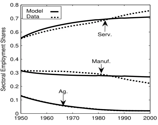
4.1. Growth and Structural Transformation for Cameroon
Cameroon had a poor economic performance between 1960 and 2000. Relative to the US,
its GDP per capita declined from 7% in 1960 to 4% in 2000. While its average growth rate
was 0.55% during the 40-year period, the path of GDP per capita shows two sub-periods
with different growth trends. The first sub-period runs from 1960 to 1983 and is
char-acterized by an average per capita GDP growth rate of 2.40%. But the growth rate was
-2.14% between 1984 and 2000. Thus, with constant productivity growth in
manufactur-ing and services, I cannot replicate the path of income per capita for Cameroon. Instead,
29
the model requires positive productivity growth rates in manufacturing and services in
the first sub-period, and negative rates in the second. The calibrated rates are 2% in
manufacturing and 1.5% in services in the first sub-period. But they were respectively
-1.8% and -4% in the second sub-period. These changes in growth rates are treated as
unexpected. That is in the first period, the household expects that the manufacturing
and service TFP growth rates will be constant for ever. After they change in 1983, the
household will believe that the new rates will be constant for ever, etc . . ..
Panel (A) of figure 2 shows the path of GDP per capita relative to 1960. The model
is able to replicate very closely the path of per capita GDP in the first sub-period but
cannot match the full decline in the second. This is due to the fact that with moderate
negative manufacturing TFP growth rate, the capital stock continues to grow albeit at
a slower rate. The graph shows that the steep decline in the second sub-period washed
away almost all the gain in income in the first sub-period. In fact, Cameroon’s GDP per
capita in 2000 was at its level in 1972.
Panel (B) shows the process of structural transformation that accompanied these 40
years of economic stagnation30. The first observation from the graph is that Cameroon
reallocated a very small percentage of its workforce out of agriculture. Agricultural
employment share declined from 78.5% to 66.2%. This implies that a major problem
for Cameroon is agricultural productivity. As long as Cameroon doesn’t improve its
productivity in agriculture, it cannot move labor to the other two sectors with higher
productivity growth. The sources of poor efficiency in the agricultural sector are diverse.
They can be the result of poor soil fertility, lack of efficient farming techniques, lack of
use of fertilizers and so on.
The second observation from the figure is that the employment share of the
manufactur-ing sector increased less compared to the increase in services. Manufacturmanufactur-ing employment
share increased from 4.6% to 9.9% while the share of services increased from 16.9% to
23.9%. This means that most of the labor reallocation occurred between the
agricul-ture and service sectors. In the model framework, the small increase in manufacturing
30
employment share is due to the low productivity of services relative to manufacturing.
Thus, the second biggest problem for Cameroon is productivity in services.
4.2. Growth and Structural Transformation for Brazil
GDP per capita for Brazil increased nearly 2.5-fold between 1960 and 2000. But the
time series shows two sub-periods with very different growth trends. From 1960 to 1980,
Brazil experienced a rapid growth with an average growth rate of 4.2%. However, Brazil
was almost stagnant between 1980 and 2000, growing on average by less than 0.8% per
year31. Despite the fast growth in the first period, Brazil did not catch up to the US. Its
GDP per capita was almost constant, around 20% of the US during the period.
Despite this mixed growth performance, Brazil experienced big changes in sectoral
em-ployment shares. Agricultural emem-ployment share decreased from 52% in 1960 to 24%
in 2000. During the same period, manufacturing employment share increased first from
15% in 1960 to 22% in 1985, and then decreased to 19% by 2000. The service
employ-ment share increased by 24 percentage points for the whole period and was at 57% in
2000. This indicates that Brazil transitioned from the first to the second phase of its
structural transformation process around 1985. One observation we can take from the
changes of labor shares is that Brazil did not allocate a large percentage of its labor force
to the manufacturing sector. One reason would be that the service sector was highly
unproductive compared to the manufacturing sector especially in the second sub-period.
Calibrating the model to match income per capita growth and the structural
trans-formation yields productivity growth rates at respectively 2.2% in manufacturing and
1.8% in services in the first sub-period. In the second sub-period, the growth rates were
respectively 1.13% and -2.4%. Again, the changes in the growth rates are treated as
unexpected and are assumed to be permanent.
With the inferred sectoral TFPs, the model is able to trace very closely the path
of per capita GDP as shown in panel (A) of figure 3. Panel (B) shows the structural
transformation of Brazil. The model is able to replicate the changes of employment
31
shares in all three sectors. We can see that the employment share of services increased
slightly more in the second sub-period than in the first. This is caused by the higher
TFP growth differential between manufacturing and services in the second sub-period.
The analysis above shows that while the agriculture and manufacturing sectors were
holding ground relative to the US, the service sector was not. In the second sub-period,
there was a dramatic decline in service TFP. This was the driving force behind income
stagnation for those 20 years. In fact, manufacturing TFP growth was high in both
sub-periods.
4.3. Growth and Structural Transformation for Korea
Korea is a growth miracle. It was able to achieve and sustain high output growth for
many years. GDP per capita increased nearly 13-fold and it was catching up to the
US. It went from 9% of the US in 1960 to 50% in 2000. It also experienced substantial
structural transformation in the period 1960-2000. The agricultural share of employment
declined from 66% in 1960 to only 10% in 2000. The manufacturing employment share
first increased from 9% in 1960 to 35% in 1991 and then declined to 28% in 2000. On
the other hand, the service share of employment increased by 37 percentage points in the
40-year period. It increased from 24% to 62% of total employment. Korea fits very well
the structural transformation process accompanying economic development as described
by Kuznets32.
The steady growth of GDP per capita from 1960 to 2000 is consistent with constant
productivity growth rates both in the manufacturing and service sectors. The calibrated
growth rates are 3.6% in manufacturing and 3.0% in services from 1960 to 2000. After
2000, I assume that these rates drop unexpectedly to the level of the US rates, implying
that the catch up of Korea stops at this time. Figure 4 shows the GDP per capita growth
and structural transformation of Korea. As can be seen in panel (A), the model replicates
very well the path of GDP per capita relative to 1960. We can also see in panel (B), the
model’s labor reallocation between manufacturing and services matches the overall trend
32
in the data but does not fit closely the time paths of sectoral employment shares33.
These two figures show that the calibrated sectoral TFP time series are consistent with
the paths of GDP per capita and sectoral employment shares for Korea. In addition, from
the model’s framework, we see that the underlying reason for Korea’s fast income growth
was the sustained increase in productivity for all three sectors. This is a key difference
with Brazil which improved productivity in all three sectors between 1960 and 1980, but
experienced a marked slowdown afterward.
4.4. Comparing Sectoral TFP Paths
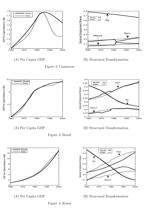
In this subsection, I summarize the paths of sectoral TFP relative to the US for the
three countries. This will highlight the least productive sectors in each country. Figure
5 plots the relative productivities in the three sectors. Panel (A) shows the relative TFP
in agriculture. Between 1960 and 1970, the US had a high TFP growth in agriculture,
therefore all other countries had downward slopping relative TFPs. However since 1970,
US agricultural TFP growth was not so high and most of the countries had increasing
relative TFPs. The highest productivity growth was for Korea, where relative TFP
more than doubled increasing from 16% in 1970 to 40% in 2000. Brazil’s relative TFP
increased somewhat after 1970 but it was only around 21% as of 2000. As I mentioned
earlier, Cameroon is very unproductive in agriculture. Its relative productivity declined
from 12% to 10% of the US in the period 1970-2000.
As can be seen in panel (B), the relative TFPs for manufacturing are higher than those
of the agriculture sector. Korea started with lower relative manufacturing TFP than
Brazil but it ended up being the highest by 2000. It increased from 36% of the US in
1960 to 85% in 2000. Brazil had high growth in the first sub-period, which slowed down
in the second. Despite of this, relative manufacturing TFP increased from 50% to 57%
in the period 1960-2000. Cameroon had a declining relative manufacturing TFP for both
subperiods with a much bigger decline in the second subperiod. Its manufacturing TFP
declined from 35% of the US in 1960 to 22% in 2000.
33
Panel (C) shows the time path of relative TFP for services . Korea experienced a
sustained growth and more than doubled its relative service TFP, increasing from 31% in
1960 to 82% in 2000. On the other end, Cameroon had a big decline in the whole period,
from 26% in 1960 to 14% in 2000. For Brazil, after a catch-up in the first sub-period, it
experienced a big decline in the second. Service TFP increased from 45% of the US in
1960 to 53% in 1980 but declined to 30% in 2000.
Comparing the relative sectoral TFPs, all countries are the least productive in
agri-culture, followed by services and then manufacturing. One way to show this is to divide
relative agricultural TFP by relative service TFP and relative service TFP by relative
manufacturing TFP. Due to a big decline of productivity in services, Cameroon’s relative
agricultural TFP increased from 68% of relative service TFP in 1960 to 74% in 2000. A
similar phenomenon occurred in Brazil where relative agricultural TFP increased from
52% of relative service TFP in 1960 to 72% in 2000. For Korea it was the opposite.
Relative TFP increased in both sectors but faster in services. Relative agricultural TFP
declined from 64% of relative service TFP in 1960 to 48% in 2000. The comparison
be-tween relative service TFP and manufacturing shows similar trends. For Cameroon and
Brazil, there were bigger declines of relative productivity for services than
manufactur-ing. Korea was catching up to the US in both sectors but with a slightly higher rate in
services. Cameroon’s relative service TFP decreased from 74% of manufacturing TFP
in 1960 to 63% in 2000. The decline was from 90% in 1960 to 52% for Brazil. Korea’s
relative service TFP increased from 86% of relative manufacturing TFP in 1960 to 97%
in 2000.
5. Discussion of the Findings
Before discussing my findings on relative sectoral TFP, I use my calculated aggregate
capital from the model to conduct a simple growth accounting for Korea and show that
the estimates are in line with studies in the growth accounting literature. Table 3 shows
grew on average at the annual rate of 6.6%, capital by 9.47% and TFP by 1.83%. The
contribution of capital to output growth was 46% while TFP contributed at 28%. In
the growth accounting literature, there is a range of estimates for the growth rate of
aggregate productivity and its contribution to output growth. The average growth rate
of TFP at different time intervals varies between 1.3% to 4.1% (see table XI in Young
(1995)). However, the consensus seems that growth of the inputs, especially capital,
contributed more to output growth. Young (1995) estimates that productivity grew on
average 1.7 % and contributed to 17% of output growth while capital contributed to
40% for the period 1966-1990. With a higher capital share, Bosworth and Collins (1996)
estimates that between 1960 and 1994, capital contributed to 58% in output per worker
growth and TFP contributed to 26%. My estimates, which don’t include the contribution
of human capital, are well within the range found in the literature.
As noted earlier, the finding that agriculture is the least productive sector in developing
countries is not new, therefore I will not discuss it here34. The interesting finding is
that relative to the US, the developing countries considered here are less productive
in services compared to manufacturing. This finding is consistent with studies that use
micro data and those that examine labor productivity. Bailey and Solow (2001) and Baily
et al. (2005) used collected data at the firm level by the McKinsey Global Institute to
compare labor productivity across sectors for few developed and developing countries35.
They find that relative to the US, other countries are less productive in services than
manufacturing. One notable example is Japan, which is more productive than the US in
many manufacturing sub-sectors (e.g. Auto, Steel, Consumer Electronics, Metalworking)
but is far behind in services. This relative productivity ranking holds true for Brazil and
Korea although Korea is very productive in some services like Telecom and Airlines.
Using a similar three-sector model without capital accumulation, Duarte and Restuccia
(2010) finds that relative to the US, other countries are less productive in agriculture,
followed by services and then industry. Their paper uses data on labor productivity from
34
See Restuccia et al. (2008); Gollin et al. (2004) for a detailed discussion of the topic. 35
the Groningen 10-sector database for 29 developed and developing countries and uses the
model to back out PPP-conversion factors across countries. Herrendorf and Valentinyi
(2007) also infers sectoral TFP across countries from a general equilibrium model. Using
relative prices obtained from the expenditure data of the 1996 benchmark studies of the
Penn World Table (PWT), they finds that relative TFP differences between the US and
developing countries are small in services compared to sectors producing consumption
goods, construction and equipment goods.
While this paper provides an innovative methodology to circumvent the data
limita-tion for sectoral productivity analysis in developing countries, it makes few assumplimita-tions.
The first is the assumption of closed economy. Following the literature on structural
transformation, this assumption is made to simplify the analysis. Moreover, the
assump-tion seems reasonable given these kind of models with a single manufacturing good, a
non tradable service sector and an agriculture sector producing only food which only a
very few developing countries trade36. As noted earlier this assumption may be strong
for countries like Korea with big manufacturing exports. However allowing for trade in
manufacturing will strengthen my results for such countries. First, there is a strong
evi-dence that only the best productive firms engage in exports. Second, the exports market
provides additional demand for the manufacturing sector which requires slow reallocation
of resources to services despite a sizeable productivity growth differential37.
Another assumption concerns the agricultural technology which uses only labor and
land with no capital, no intermediate inputs and no distortions. Indeed there are a
number of papers that indicate these are important to explain the low productivity in
agriculture. While extending the model to include any of these will have a quantitative
effect on agricultural TFP, it will not alter the finding that agriculture is the least
pro-ductive sector which is very robust finding of the development literature. Also it will not
affect the sectoral TFPs for the other two sectors because what is critical for their
de-termination is to have the correct level of non-agricultural labor; capital is endogenously
36
Gollin et al. (2007) used data from Food and Agriculture Organization (FAO) and concluded that only a few developing countries engage in food trade.
37
determined. The model also makes the assumption of no dual labor market and wages
are equalized across sectors. If the duality of the labor market is between agriculture
and non-agriculture, then the above argument applies. However, there is some evidence
that wages in some service sub-sectors (like retail) are lower than those in manufacturing.
This model is too aggregated to deal with such an issue. Another interesting departure
is to have different kind of labor (skilled vs unskilled). Future work will address these
issues.
6. Conclusion
This paper shows that we can use time series data on sectoral employment shares and
GDP per capita to infer time series of sectoral TFP. The proposed approach develops
a three-sector model where non-homothetic preferences and differences in sectoral
pro-ductivity drive labor reallocation across sectors. In this framework, labor moves to the
slowest growing sectors. The model is calibrated to the US and is shown to replicate the
structural transformation process of the US economy for the period 1950-2000. Applying
the calibrated model to developing countries leads to the interesting finding that relative
to the US, developing countries are the least productive in services compared to
manufac-turing. This finding results from the fact that the countries allocate a greater percentage
of their labor force to the service sector rather than manufacturing.
A key innovation of this paper is the use of panel data on sectoral employment and GDP
per capita, which allows us to compute time series for sectoral TFPs. This is important
because many developing countries experience large changes in GDP growth over time
which suggests that their sectoral TFPs undergo large changes over time as well. With
long time series, we can find not only the least productive sectors in developing countries,
but also the sectoral sources of big changes in GDP per capita for a given country.
While sectoral TFP growth differentials and non-homotheticity have been the key
driv-ing forces of labor reallocation in this model, such reallocation can also be the result of
need to understand how and why policies and institutions affect sectors differently. These
questions are left for future research.
References
Adamopoulos, Tasso and Ahmet Akyol, “Relative Underperformance Alla Turca,”
Review of Economic Dynamics, 2009, 12(1), 697–717.
Bah, Elhadj M., “Structural Transformation in Developed and Developing Countries,”
2009. The University of Auckland Working Paper.
and Josef C. Brada, “Total Factor Productivity, Structural Change and Convergence
in Transition Econmies,” Comaprative Economic Studies, 2009, 51(4), 421–446.
Bailey, Martin McNeil and Robert M. Solow, “International Productivity
Com-parisons Built From the Firm Level,” Journal of Economic Perspectives, 2001, 15 (3),
151–172.
Baily, Martin, Diana Farrell, and Jaana Remes, “Domestic Services: The Hidden
Key to Growth,” 2005. The McKinsey Global Institutes.
Beaumol, William, “Macroeconomics of Unbalanced Growth: The anatomy of Urban
Crisis,”The American Economic Review, 1967, 57 (3), 415–426.
Bosworth, Barry P. and Susan M. Collins, “The Economic Growth in East Asia:
Accumulation Versus Assimilation,” Brookings Papers on Economic Activity, 1996,27
(2), 135–204.
Brauer, David, “What account for the Decline in Manufacturing Employment?,” 2006.
Economic and budget issue brief.
Caselli, Francesco, “Accounting for Cross-Country Income Diferences,” in Philippe
Chanda, Areendam and Carl-Johan Dalgaard, “Dual Economies and International
Total Factor Productivity Differences,” 2005. Louisina State University Working Paper.
Duarte, Margarida and Diego Restuccia, “The Role of Structural Transformation
in Aggregate Productivity,” Quaterly Journal of Economics, forthcoming, 2010, 125
(1).
Echevarria, Christina, “Changes in Sectoral Composition Associated with Economic
Growth,”International Economic Review, 1997,38 (2), 431–452.
Gollin, Douglas, “Getting Income Shares Right,” Journal of Political Economy, 2002,
110(2), 458–474.
, Stephen L. Parente, and Richard Rogerson, “The Role of Agriculture in
Devel-opment,”American Economic Review: Papers and Proceedings, 2002,92 (2), 160–164.
, , and , “Farmwork, Homework and International Income Differences,” Review
of Economic Dynamics, 2004,7 (4), 827–850.
, , and , “The Food Problem and the Evolution of International Income Levels,”
Journal of Monetary Economics, 2007, 54 (4), 1230–1255.
Hall, Robert E. and Charles I. Jones, “Why do Some Countries Produce So Much
More Output per Worker than Others,”The Quaterly Journal of Economics, 1999,114
(1), 83–116.
Hayami, Yujiro and Vernon W. Ruttan, “Agricultural Differences Among
Coun-tries,”The American Economic Review, 1970, 60 (5), 895–911.
and , Agricultural Development: An International Perspective, Baltimore: John Hopkins, 1985.
Hendricks, Lutz, “How Important is Human Capital for Development? Evidence from
Herrendorf, Berthold and Akos Valentinyi, “Which Sector Make the Poor Countries
So Unproductive,” 2007. Arizona State University working paper.
and , “Measuring Factor Income Shares at the Sectoral Level,”Review of Economic
Dynamics, 2008, 11(4), 820–835.
Hsieh, Chang-Tai and Peter J. Klenow, “Relative Prices and Relative Prosperity,”
The American Economic Review, 2007,97 (3), 562–585.
Klenow, Peter J. and Andres Rodriguez-Clare, “The Neoclassical Revival in
Growth Economics: Has It Gone Too Far?,” in Ben Bernanke and Julio J.
Rotem-berg, eds.,NBER Macroeconomics Annual, MIT Press 1997, pp. 73–103.
Kongsamut, Piyabha, Sergio Rebelo, and Danyang Xie, “Beyond Balanced
Growth,”Review of Economic Studies, 2001,68 (4), 869–882.
Kuznets, Simon, Economic Growth of Nations, Cambridge: Harvard University Press,
1971.
Laitner, John, “Structural Change and Economic Growth,”Review of Economic
Stud-ies, 2000, 67 (3), 545–561.
Maddison, Angus, “Historical Statistics of the World Economy: 1-2006 AD,” http:
//www.ggdc.net/Maddison 2009.
Mundlank, Yair, “Production and Supply,” in B. Gardner and G. Rausser, eds.,
Hand-book of Agricultural Economics, Vol. I, Amsterdam: Elsevier, 2001, pp. 3–85.
Ngai, L. Rachel and Christopher A. Pissarides, “Structural Change in a
Multi-Sector Model of Growth,” American Economic Review, 2007,97 (1), 429–443.
Parente, Stephen L. and Edward C. Prescott, “Barriers to Technology Adoption
and Development,”Journal of Political Economy, 1994,102 (2), 298–321.
Prescott, Edward C., “Needed: A theory of Total Factor Productivity,” International Economic Review, 1998,39 (3), 525–551.
Restuccia, Diego, Dennis Tao Yang, and Xiadong Zhu, “Agriculture and
Aggre-gate Productivty: A Quantitative Cross-Country Analysis,”The Journal of Monetary
Economics, 2008, 55 (2), 234–250.
Rogerson, Richard, “Structural Transformation and the Deterioration of European
Labor Market Outcomes,” Journal of Political Economy, 2008, 116 (2), 235–259.
Sachs, Jeffrey and Andrew Warner, “Economic Reform and the Process of Global
Integration,”Brooking Papers on Economic Activity, 1995,1995 (1), 1–118.
Vollrath, Dietrich, “Relative Underperformance Alla Turca,”Journal of Development
Economics, 2009, 88 (1), 325–334.
Wacziarg, Romain and Karen Horn Welch, “Trade Liberalization and Growth:
New Evidence,” World Bank Economic Review, 2008,22 (2).
Young, Alwyn, “The Tyranny of Numbers: Confronting the Statistical Realities of the
East Asian Growth Experience,” The Quaterly Journal of Economics, 1995, 110 (3),
641–680.
, “Endogenous TFP and Cross-Country Income Differences,” Journal of Monetary
Economics, 2008, 55 (6), 1158–1170.
A. Appendix A: Data Sources
The calibration of the model to the US economy requires data for GDP per capita, sectoral
shares of hours worked, price of services relative to manufacturing, investment to output
and capital to output. The data for GDP per capita, expressed in 1990 international
Geary-Khamis dollars, is from the “Historical Statistics for the World Economy: 1-2006
relative to manufacturing are from the Groningen 10-sector database. In the database, the
economy is disaggregated into 10 sectors. The value-added of each sector is given in both
constant and current prices. I aggregated those sectors into the 3 sectors used throughout
this paper. Manufacturing includes mining, manufacturing, utilities and construction. I
calculate the price of a sector by dividing its value added in current prices by the value
added in constant prices. The price of services relative to manufacturing is deduced form
there. This database also contains the sectoral hours worked for the US between 1950
and 1997. For the period, 1998-2000, I use the 60-sector industry database. I obtained
investment series from the NIPA tables and used the perpetual inventory method to
calculate capital stocks.
For the application of the model to the developing countries, I need data on sectoral
employment and GDP per capita. The employment shares data is obtained from the
World Bank tables (1983) for the years 1960, 1965 and 1970 and World Development
Indicators online database from 1971. The per capita GDP is from Maddison.
The GDP per capita and sectoral employment shares data series for the US and
devel-oping countries have been filtered using the H-P filter to focus on low frequency trends.
B. Appendix B: Figures, Proofs and Tables
B.1. Proofs
Proof 1: Deriving equation for the non-agricultural aggregate expenditure Ct
Ct =Mt+pstSt (31)
Using equation (24) yields:
Ct=Mt+
Amt
Ast
St (32)
We also know that Φt(Mt, St) is homogenous of degree 1, therefore:
Φ1 =λM −1 ǫ t ϕ 1 ǫ t (34)
Φ2 = (1−λ)S
−1 ǫ t ϕ 1 ǫ t (35)
But from equation (17), we have:
1−λ
λ
Mt
St
1ǫ
= Amt
Ast
(36)
Then:
Φ2 =
Amt
Ast
Φ1 (37)
This implies:
Φt = Φ1M1+
Amt
Ast
Φ1St= Φ1
Mt+
Amt
Ast
St
= Φ1Ct (38)
Replacing Φ1 by its expression, yields:
Ct=
ϕtM
1
ǫ
t
λ (39)
where ϕt is as defined in 15
Proof 2: Deriving the dynamic equation for capital
From equations (32) and (18):
Ct=Mt+Amt
Kt
Nt
θ
Nst (40)
Then:
Ct =Amt
Kmt
Nmt
θ
Nmt+ (1−δ)Kt−Kt+1+Amt
Kt
Nt
θ
Nst (41)
Since Kmt
Nmt =
Kt
Nt, this reduces to:
Ct=Amt
Kt
Nt
θ
This implies:
Kt+1 =Amt
Kt
Nt
θ
Nt+ (1−δ)Kt−Ct (43)
Combining equations (19) and (43), we get the following dynamic equation for the
ag-gregate capital stock:
Kt+1 = Amt
Kt
Nt
θ
Nt+ (1−δ)Kt−β
"
1−δ+θAmt
Kt
Nt
θ−1#
" Amt−1
Kt−1
Nt−1
θ
Nt−1+ (1−δ)Kt−1−Kt
#
(44)
Proof 3: Deriving labor used in services
From equations (17) and (16), we have:
Mt=Amt
λ
1−λ
ǫ Ast
Amt
1−ǫ
Kt
Nt
θ
Nst (45)
Combining equations (40) and (45), we get:
Ct=Mt+Amt
Kt
Nt
θ
Nst =Amt
Kt Nt θ" 1 + λ
1−λ
ǫ Ast
Amt
1−ǫ#
Nst (46)
From equation (46) we can get the quantity of labor used in the service sector.
Nst =
Ct Amt Kt Nt θ
1 + 1−λλ
ǫAst
Amt
1−ǫ (47)
[image:34.595.99.495.672.748.2]B.2. Figures and Tables
Table 1: Statistics in the Data and the Model
Statistics, average 1950-2000 Data (%) Model (%)
Per Capita GDP Growth Rate 2.10 2.10
Capital to Output Ratio 2.40 2.40
Investment to Output Share 20.30 20.70
Table 2: Calibrated Parameters
Aa Am As A α β δ ǫ λ θ γm γs
[image:35.595.148.445.282.391.2]1 1 1 0.24 0.7 0.97 0.04 0.45 0.01 0.33 0.014 0.0052
Table 3: Growth Accounting for Korea
Annual growth rate Contribution to output
Output 0.0667 1.00
Capital 0.0947 0.47
Labor 0.0251 0.25
TFP 0.0183 0.28
NOTE: The output is for the non-agricultural sectors.
19500 1960 1970 1980 1990 2000
0.1 0.2 0.3 0.4 0.5 0.6 0.7 0.8
Sectoral Employment Shares
Model Data
Ag.
Manuf. Serv.
[image:35.595.153.426.495.711.2]19601 1970 1980 1990 2000 1.1 1.2 1.3 1.4 1.5 1.6 1.7 1.8
GDP Per Capita Relative to 1960
Model Data
(A) Per Capita GDP
19600 1970 1980 1990 2000 0.1 0.2 0.3 0.4 0.5 0.6 0.7 0.8
Sectoral Employment Shares
Manuf.
Serv. Ag.
Model Data
[image:36.595.64.562.53.788.2](B) Structural Transformation
Figure 2: Cameroon
19601 1970 1980 1990 2000 1.5
2 2.5
GDP Per Capita Relative to 1960
Model Data
(A) Per Capita GDP
1960 1970 1980 1990 2000 0.1 0.15 0.2 0.25 0.3 0.35 0.4 0.45 0.5 0.55 0.6
Sectoral Employment Shares
Model
Data Serv.
Ag.
Manuf.
[image:36.595.337.554.86.235.2](B) Structural Transformation
Figure 3: Brazil
19600 1970 1980 1990 2000 2 4 6 8 10 12 14
GDP Per Capita Relative to 1960
Model Data
(A) Per Capita GDP
19600 1970 1980 1990 2000 0.1 0.2 0.3 0.4 0.5 0.6 0.7
Sectoral Employment Shares
Model Data
Ag.
Serv.
Manuf.
(B) Structural Transformation
[image:36.595.336.539.558.709.2]1960 1970 1980 1990 2000 0.1
0.15 0.2 0.25 0.3 0.35 0.4 0.45 0.5
Agricultural TFP Relative to the US
Cameroon
Brazil Korea
(A) Agriculture
1960 1970 1980 1990 2000 0.2
0.3 0.4 0.5 0.6 0.7 0.8 0.9 1
Manufacturing TFP Relative to the US
Cameroon
Brazil
Korea
(B) Manufacturing
1970 1980 1990 2000 0.1
0.2 0.3 0.4 0.5 0.6 0.7 0.8 0.9
Service TFP Relative to the US
Cameroon Brazil
Korea
[image:37.595.68.507.201.664.2](C) Services