Overcoming the problem of multicollinearity in sports performance data: A novel application of partial least squares correlation analysis

(2019) Overcoming the problem of multicollinearity in sports performance data: A novel application of partial least squares correlation analysis. PLoS ONE. ISSN 1932-6203 DOI: https://doi.org/10.1371/journal.pone.0211776

Link to Leeds Beckett Repository record:

http://eprints.leedsbeckett.ac.uk/5713/

Document Version: Article

Creative Commons: Attribution 4.0

The aim of the Leeds Beckett Repository is to provide open access to our research, as required by funder policies and permitted by publishers and copyright law.

The Leeds Beckett repository holds a wide range of publications, each of which has been checked for copyright and the relevant embargo period has been applied by the Research Services team.

We operate on a standard take-down policy. If you are the author or publisher of an output and you would like it removed from the repository, please contact us and we will investigate on a case-by-case basis.

Overcoming the problem of multicollinearity

in sports performance data: A novel

application of partial least squares correlation

analysis

Dan WeavingID1,2*, Ben Jones1,3,4, Matt Ireton1,5, Sarah WhiteheadID1,2, Kevin Till1,2,3,

Clive B. Beggs1

1 Institute for Sport, Physical Activity and Leisure, Leeds Beckett University, Leeds, West Yorkshire, United Kingdom, 2 Leeds Rhinos Rugby League club, Leeds, United Kingdom, 3 Yorkshire Carnegie Rugby Union club, Leeds, United Kingdom, 4 The Rugby Football League, Leeds, United Kingdom, 5 Warrington Wolves Rugby League club, Warrington, United Kingdom

*[email protected]

Abstract

Objectives

Professional sporting organisations invest considerable resources collecting and analysing data in order to better understand the factors that influence performance. Recent advances in non-invasive technologies, such as global positioning systems (GPS), mean that large volumes of data are now readily available to coaches and sport scientists. However analys-ing such data can be challenganalys-ing, particularly when sample sizes are small and data sets contain multiple highly correlated variables, as is often the case in a sporting context. Multi-collinearity in particular, if not treated appropriately, can be problematic and might lead to erroneous conclusions. In this paper we present a novel ‘leave one variable out’ (LOVO) partial least squares correlation analysis (PLSCA) methodology, designed to overcome the problem of multicollinearity, and show how this can be used to identify the training load (TL) variables that influence most ‘end fitness’ in young rugby league players.

Methods

The accumulated TL of sixteen male professional youth rugby league players (17.7±0.9 years) was quantified via GPS, a micro-electrical-mechanical-system (MEMS), and players’ session-rating-of-perceived-exertion (sRPE) over a 6-week pre-season training period. Immediately prior to and following this training period, participants undertook a 30–15 inter-mittent fitness test (30-15IFT), which was used to determine a players ‘starting fitness’ and

‘end fitness’. In total twelve TL variables were collected, and these along with ‘starting fit-ness’ as a covariate were regressed against ‘end fitfit-ness’. However, considerable multicolli-nearity in the data (VIF>1000 for nine variables) meant that the multiple linear regression (MLR) process was unstable and so we developed a novel LOVO PLSCA adaptation to quantify the relative importance of the predictor variables and thus minimise multicollinearity

a1111111111 a1111111111 a1111111111 a1111111111 a1111111111

OPEN ACCESS

Citation: Weaving D, Jones B, Ireton M, Whitehead S, Till K, Beggs CB (2019) Overcoming the problem of multicollinearity in sports performance data: A novel application of partial least squares correlation analysis. PLoS ONE 14(2): e0211776.https://doi. org/10.1371/journal.pone.0211776

Editor: Chris Connaboy, University of Pittsburgh, UNITED STATES

Received: June 18, 2018

Accepted: January 22, 2019

Published: February 14, 2019

Copyright:©2019 Weaving et al. This is an open access article distributed under the terms of the Creative Commons Attribution License, which permits unrestricted use, distribution, and reproduction in any medium, provided the original author and source are credited.

Data Availability Statement: All relevant data are within the paper (Table 1andTable 2).

issues. As such, the LOVO PLSCA was used as a tool to inform and refine the MLR process.

Results

The LOVO PLSCA identified the distance accumulated at very-high speed (>7 m�s-1) as being the most important TL variable to influence improvement in player fitness, with this variable causing the largest decrease in singular value inertia (5.93). When included in a refined linear regression model, this variable, along with ‘starting fitness’ as a covariate, explained 73% of the variance in v30-15IFT‘end fitness’ (p<0.001) and eliminated

completely any multicollinearity issues.

Conclusions

The LOVO PLSCA technique appears to be a useful tool for evaluating the relative impor-tance of predictor variables in data sets that exhibit considerable multicollinearity. When used as a filtering tool, LOVO PLSCA produced a MLR model that demonstrated a signifi-cant relationship between ‘end fitness’ and the predictor variable ‘accumulated distance at very-high speed’ when ‘starting fitness’ was included as a covariate. As such, LOVO PLSCA may be a useful tool for sport scientists and coaches seeking to analyse data sets obtained using GPS and MEMS technologies.

Introduction

Professional sporting organisations invest considerable resources collecting and analysing data to better understand the factors that influence athletic performance. Recent advances in wearable technology and computing power mean that large volumes of data are now readily available to

the applied practitioner [1]. However, while this data is becoming easier to collect, analysing it

can be a challenging task, particularly when sample sizes are small (i.e. limited by squad size) and the data is highly correlated–something that can lead to instability when applying standard least

squares regression techniques, making it difficult to draw firm inference [2–3]. With respect to

this, global positioning system (GPS) and micro-electrical-mechanical-system (MEMS) data can

be particularly problematic [4–5]. GPS and MEMS are often used to measure an athlete’s

move-ment, from which speed, distance travelled, and acceleration can be computed using standard mathematical algorithms. For example, a player’s velocity and acceleration are simply the first and second derivatives of the distance travelled. Consequently, these variables are not indepen-dent, but instead are highly correlated. It is therefore not surprising that strong correlations have

been reported between variables widely used to assess training load (TL) [4–5].

Whilst individual measured variables are collected when acquiring performance data, these are often grouped together to represent latent constructs such as ‘fitness’, ‘fatigue’ or ‘techni-cal-tactical performance’. For example, a rugby league coach might represent ‘attacking perfor-mance’ using variables such as the ‘number of metres run’, ‘tackle breaks’ or ‘kick return

metres’ [6]. Conversely, a sports scientist might assess the TL imposed using data acquired

from GPS or MEMS [4]. However, quantifying the relationships within and between these

var-ious latent constructs can be challenging because the individual variables used to quantify, for example, TL in athletes, have been shown in a meta-analysis to possess substantial correlations

[5], making them prone to multicollinearity issues [3,5]. Nevertheless, when attempting to

understand relationships between the latent constructs used in sports performance,

preparation of the manuscript. The specific roles of these authors are articulated in the ‘author contributions’ section.

multicollinearity issues are often ignored, with the tendency being instead to rely on univariate

analysis [7–10]. However, univariate analysis has the inherent drawback that it assumes that

the variables are independent and does not allow for any covariance within the data, some-thing that can be a major weakness. Furthermore, it is not possible using univariate analysis to ‘capture’ any information that may be associated with the covariance between the variables, something that might be particularly important when considering the effect that changes in prescribed training mode across a training period might have on the relationships between TL

variables [4–5,11–12]. Consequently, when analysing TL data it is important to allow for

covariance in the data in order to ensure that appropriate inference is drawn and that errone-ous conclusions are not reached.

When more sophisticated analysis is used, multiple linear regression (MLR) is generally the tool used by practitioners to quantify the strength of relationships within TL data. It is common practice when performing MLR to retain only those predictor variables that ‘confidently explain’ the behaviour of the response (dependent) variable, with variables that fail to reach a required level of significance excluded. While this approach works well when the predictor vari-ables are weakly correlated with each other, problems can occur when strong correlations are

present and variable inflation factors (VIFs) are>10 [13–15]. Multicollinearity over-inflates the

standard errors associated with the respective regression coefficients, causing the p-values to become very sensitive to changes in model specification, resulting in the whole process becom-ing unstable. Consequently, multiple competbecom-ing models may be produced, makbecom-ing it difficult to

be confident about any inference drawn from the various models [2]. In contrast to MLR,

singu-lar value decomposition (SVD) is immune to multicollinearity because it produces a set of

orthogonal composite variables that are completely uncorrelated [16–18]. Although not a

statis-tical techniqueper se, SVD underpins other techniques such as principal component analysis

(PCA) and partial least squares correlation analysis (PLSCA) [19–20]. PLSCA in particular

appears to have considerable potential with regard to the analysis of small data sets that exhibit multicollinearity (e.g. sports performance data sets). Because PLSCA incorporates SVD, it has the great advantage that it is both immune to multicollinearity, and unlike MLR, can cope with situations where the number of predictor variables exceeds the number of observations. Unlike MLR, which involves one response (dependent) variable and multiple predictor (independent) variables, PLSCA sub-divides the data into two blocks (sub-groups) each containing one or more variables, and then uses SVD to establish the strength of any relationship that might exist

between the two component sub-groups [21]. It does this by using SVD to determine the inertia

(sum of the singular values) of the covariance matrix of the sub-groups under consideration

[17,19,21]. Given that the singular values are proportional to the magnitude of any effect [17],

the higher the value of the singular value inertia observed, the greater the amount of shared information between the respective sub-groups and the stronger the relationship between the two. PLSCA is usually accompanied by a one-tailed permutation test generally involving 10,000 random permutations in order to establish the null distribution of the possible inertias and the

likelihood (the odds) of the observed relationship occurring by chance [21].

Although PLSCA has been widely used in neuroimaging [17,19–20,22], it has not been used

in sport science, with the result that its potential in this discipline has not been exploited. We therefore hypothesised that PLSCA might be a useful tool with which to analyse small sport performance data sets. As sport scientists regularly seek to identify the TL variables that best relate to training outcome measures, we designed the study presented here with the aim of investigating the relationship between the accumulation of TL (quantified using multiple

col-lection methods), and 30–15 intermittent fitness test (30-15IFT) performance achieved by 16

(LOVO)’ adaptation, might be a useful tool for analysing TL data sets where multicollinearity issues are problematic. More specifically, we wanted to know if the above methodology could

identify which accumulated TL variables best relate to 30-15IFTperformance following

6-weeks of training.

Leave one variable out PLSCA example

In order to explain the linear algebra underpinning PLSCA and to highlight the LOVO

adapta-tion, we shall first consider a small dataset (Table 1) containing publicly available data collected

from the twelve teams competing in the European Super League during the 2017 season

(https://rugby-league.com/superleague/stats/club_stats). In this data set we have two outcome

variables for the season: total league points accumulated and total match score difference; and three performance related variables: the number of missed tackles; the number of tackle busts; and the number of clean breaks. If for example, we wanted to establish whether or not a rela-tionship exists between these two groups of variables, we could perform PLSCA to assess the amount of shared information common to the two and use this to quantify the strength of any relationship.

PLSCA is generally performed by first mean centring and standardizing the data to unit

variance [23] and then dividing it into two matrices, in this case a [12×2] matrix,X, containing

the variables total league points accumulated and total score difference, and a [12×3] matrix,

Y, containing the number of missed tackles, the number of tackle busts, and the number of

clean breaks. The pattern of relationships between the columns ofXandYcan be stored in a

[3×2] covariance matrix,R, [21] which is computed as follows:

R¼YT_X¼

0:770 1:765 2:200

0:007 0:465 0:433

0:161 0:591 0:248

0:796 0:827 0:124

0:818 0:580 0:542

0:746 0:337 0:727

0:820 0:049 0:898

0:782 1:275 0:820

1:897 0:090 0:170

0:617 1:561 0:155

0:772 1:348 1:222

1:631 0:548 1:547

2 6 6 6 6 6 6 6 6 6 6 6 6 6 6 6 6 6 6 6 6 6 6 6 6 6 6 6 6 4 3 7 7 7 7 7 7 7 7 7 7 7 7 7 7 7 7 7 7 7 7 7 7 7 7 7 7 7 7 5 T �

2:104 2:274

0:866 0:405

0:000 0:079

0:371 0:906

0:371 0:328

0:371 0:405

0:248 0:162

0:495 0:115

0:248 0:162

0:495 0:115

0:248 0:103

1:362 0:026

2 6 6 6 6 6 6 6 6 6 6 6 6 6 6 6 6 6 6 6 6 6 6 6 6 6 6 6 6 4 3 7 7 7 7 7 7 7 7 7 7 7 7 7 7 7 7 7 7 7 7 7 7 7 7 7 7 7 7 5 ¼

2:984 1:864

8:985 6:408

8:739 9:043

2 6 6 4 3 7 7 5ð1Þ

SVD of the matrix,R, yields three orthogonal matrices: a [3×2] left singular vector matrix,

U, containing the saliences (weights) for matrix,Y; a [2×2] right singular vector matrix,V,

con-taining the saliences (weights) for matrix,X; andS, a [2×2] diagonal matrix containing the

sin-gular values [21].

R¼USVT_¼

0:204 0:342

0:645 0:658

0:736 0:671

2 6 6 4 3 7 7 5�

17:021 0:000

0:000 1:617

" #

� 0:754 0:656

0:656 0:754

" #T

ð2Þ

computing the inertia,ø, (i.e. the sum of all the non-zero singular values) common to the two

sub-groups, as follows [21]:

φ¼X n

i

si ¼17:021þ1:617¼18:638 ð3Þ

where;nis the number of non-zero singular values of matrixR; andsiisithdiagonal element of

matrixS. Singular value inertia is an effect size, which directly relates to the strength of the

relationship between the two sub-groupsXandY(i.e. the greater the magnitude of the inertia

to more shared information common toXandY).

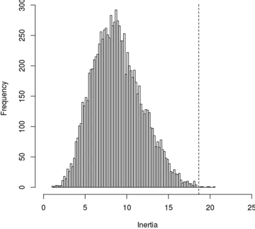
The statistical significance of the calculated inertia value can then be assessed using a

permutation test in which the rows ofYare randomly permutated 10,000 times [21], to

produce the null distribution of all the possible inertia values that could occur just by

chance, as shown inFig 1. From this it can be seen that an inertia value of�18.638 only

occurred 11 times in 10,000 simulations. This equates to a p-value of 0.0011 and indicates that, perhaps unsurprisingly, a very strong relationship exists between the match perfor-mance and season outcome variables, something that is unlikely to have occurred by chance.

Having established that a strong relationship exists between the performance variables and season outcome, it is possible to interrogate the data further to identify which variables are most influential. In order to do this in a systematic manner, we developed a novel

LOVO strategy, mirroring similar approaches adopted for SVD [18] and random forests

[23], which involved repeating the PLSCA several times, with a differentYvariable excluded

from the analysis on each occasion. By observing the effect of each successive omission on the magnitude of the inertia, it is possible to assess the relative contribution of each perfor-mance variable to league outcome. In the example above, when the ‘number of missed tack-les’ is omitted from the analysis, the inertia falls only marginally to 18.178, suggesting that this variable is not particularly influential. However by comparison, when the ‘number of tackle busts’ and the ‘number of clean breaks’ are omitted, then the inertia falls to 13.854 and 11.786 respectively, indicating that these two variables are much stronger predictors of league outcome.

Materials and methods

Participants

An observational research study was conducted in which the accumulated TL of sixteen male

professional youth rugby league players (age [y]: 17.7±0.9; height [cm]: 179.6±5.5; body

mass [kg]: 87.0±8.8) was quantified via GPS, MEMS and session-rating-of-perceived-exertion

(sRPE) during a 6-week pre-season training period. Immediately prior to and following this

training period, participants undertook the 30–15 intermittent fitness test (30-15IFT), which

was used to determine a players ‘starting fitness’ and ‘end fitness’. The content of the training and testing periods was prescribed by the coaching staff and included 3 to 4 field-based ses-sions per week comprising technical-, tactical-, sprint-, interval- and small-sided-games-based-training. The total number of recorded field training sessions was 273 with players

par-ticipating in 17±3 sessions. All procedures performed in the study were in accordance with

Procedures

The 30-15IFTwas conducted on artificial turf following two days of complete rest and prior to

any additional training as per previous methods [24]. Players possessed familiarity with the

30-15IFTas part of their regular monitoring practices. The 30-15IFTcomprised 30 second shuttles

run over 40m, with 15 seconds of recovery. The speed of the test was controlled by an audible sound. At this time of the sound, players were required to be within a 3 m tolerance zone at

either end or the middle of the 40 m shuttle. The start speed of the test was 8 km�h-1and

increased by 0.5 km�h-1following each successive shuttle. The test terminated when players

were no longer able to maintain the required speed of the test or when they did not reach the 3 m tolerance zone on three consecutive occasions. The last completed velocity during the test

Fig 1. Singular value inertial value (indicated by dotted line) computed from the observed data and the null-distribution of the inertia computed using a permutation test with 10,000 permutations.

was taken as v30-15IFT. The v30-15IFTachieved prior to the start of the training period was

deemed to be each players ‘starting fitness’ whilst the v30-15IFTachieved at the completion of

the six-week training period was deemed to be each players ‘end fitness’.

All external training load measures were collected concurrently during each training ses-sion using 10 Hz GPS devices with in-built 100 Hz tri-axial accelerometer, gyroscope and mag-netometer (Optimeye S5, Catapult Innovations, Melbourne, Victoria; firmware version: 7.17). This data was downloaded into specialist software (Catapult Sprint v5.1.7, Catapult Innova-tions, Melbourne, Victoria). The device was positioned between the scapulae within a manu-facturer designed vest according to typical procedures. Each player wore the same unit for

each session to limit potential between-unit variability in the data collected [25]. The mean

number of satellites and horizontal dilution of precision (HDOP) during the data collection

period was 15±3 and 0.8±0.6 respectively [25].

Derived from GPS, the total distance (m) covered during the ~17 training sessions was fur-ther differentiated into the distances (m) covered at arbitrary speed thresholds of low- (0 to 3

m�s-1; SZ1), moderate- (3.1 to 5 m�s-1; SVZ2), high- (5.1 to 7 m�s-1; SZ3) and very-high-speeds

(>7.1 m�s-1; SZ4). The minimum effort duration for each of the speed zones were set at 1

sec-ond [26]. An individualised high-speed threshold (IndSZ) was also calculated for each player,

which was defined as the distance covered above the terminal speed achieved during the

30-15IFTprior to commencement of the training programme. Between the players, this speed

threshold ranged from 4.58 to 5.41 m�s-1.

Derived from the tri-axial accelerometer, total session PlayerLoad is a modified vector mag-nitude and is expressed as the square root of the sum of the squared instantaneous rate of

change in acceleration in each of the three axes (X, Y, and Z) and divided by 100 [27]. This was

further differentiated into four zones relating to low- (0 to 1 AU; PLZ1), moderate- (1.1 to 2

AU; PLZ2), high- (2.1 to 3 AU; PLZ3) and very-high (>3 AU; PLZ4) accumulation of

Player-Load. All PlayerLoad variables were expressed in arbitrary units (AU). PlayerLoad has

previ-ously been shown to possess acceptable reliability [27]. sRPE was calculated for each player

during the study period using the method of Foster et al. [28]. Exercise intensity for sRPE was

determined using the Borg category ratio-10 scale, with players providing this ~15 to 30

min-utes following the cessation of the session [28]. This was then multiplied by the

training-ses-sion duration to calculate the sRPE training load in AU.

Statistical analysis

In order to assess the strength of the relationships between the variables, we first undertook Pearson correlation analysis and then performed MLR analysis with ‘end fitness’ as the response variable and all the other variables included as predictors. VIF values were then

cal-culated for each of the respective predictor variables, with those>10 identified as being

partic-ularly problematic [13–15].

inertia and p value noted. This process was repeated with a different predictor variable omitted each time (as described above), until the contribution of all the variables had been evaluated individually. Having done this, those variables that were deemed influential were used to con-struct refined PLSCA and MLR models. Improvements derived from refining the baseline PLSCA model were assessed using the Chi- square test and Cramer’s V. MLR analysis was per-formed with ’end fitness’ as the response variable and ’starting fitness’ as a covariate, as

recom-mended by Allison [29]. All analysis was undertaken using a combination of in-house

algorithms written in Matlab (version R2016b: utilising the ‘Statistics and machine learning’ toolbox) (Math-Works, Natick, MA) and R (version 3.3.2: utilising the packages: ‘psych’; ‘car’;

and ‘pracma’) (open source software). For all analyses, p values<0.05 were deemed

significant.

Results

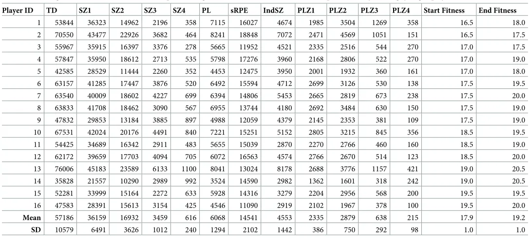
The TL descriptive results are presented inTable 2along with the study data collected for each

of the 16 subjects.

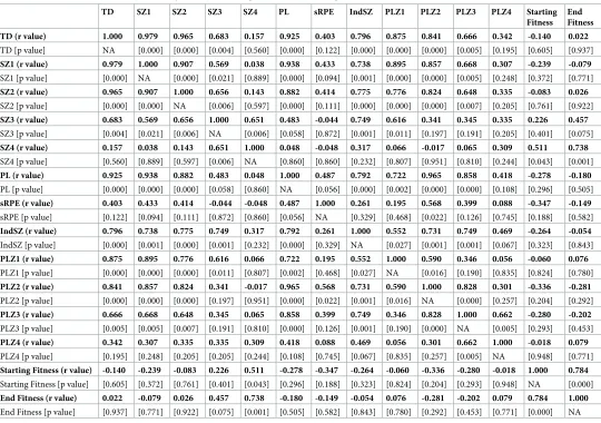
Pearson correlation analysis (Table 3) revealed multiple strong correlations between the

predictor variables in the data, suggesting that the data exhibited considerable multicollinear-ity, something that was confirmed by the extremely high VIF values obtained when MLR

anal-ysis was performed (Table 4). FromTable 4it can be seen that all but one (i.e. sRPE) of the

predictor variables exhibited a VIF>10, with most having values>1000. However, despite

numerous strong relationships in the data, ‘end fitness’ was only significantly positively

corre-lated with the variables ‘SZ4’ (r = 0.738, p = 0.001) and ‘starting fitness’ (r = 0.784, p<0.001)

(Table 3).

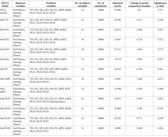
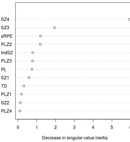
The results of the LOVO PLSCA (Table 5) revealed that the greatest decrease in measured

(computed) inertia compared with baseline occurred when the variables SZ3 (1.945) and SZ4 (5.926) were omitted from the PLSCA model, indicating that these were the most influential

variables, as illustrated byFig 2. When only these predictor variables were used to construct

the PLSCA model (Table 6), the p value achieved was 0.015, indicating that the matrix

contain-ing the predictor variables SZ3 and SZ4 shared a considerable amount of information with the output matrix containing the variables ‘starting fitness’ and ‘end fitness’ and that therefore they were likely to be the best predictors of end fitness. Given that ‘starting fitness’ can be

Table 1. League outcome and match performance data for the teams in the European Super League (season 2017).

Team League Points Score difference Number

of missed tackles

Number of tackle busts

Number of clean breaks

Castleford Tigers 40 391 1523 918 208

Leeds Rhinos 30 76 1588 796 153

Wigan Warriors 23 21 1574 697 157

Warrington Wolves 20 -145 1654 830 165

Wakefield Trinity Wildcats 26 63 1519 698 174

Salford Red Devils 26 76 1525 784 178

Huddersfield Giants 21 35 1656 757 143

Hull FC 27 27 1522 872 180

St Helens 25 25 1746 744 166

Leigh Centurions 12 12 1639 606 159

Widnes Vikings 11 -269 1652 626 136

Catalans Dragons 15 -220 1451 701 129

treated as a covariate, this implies that SZ3 and SZ4 were likely to be the best predictors of end fitness.

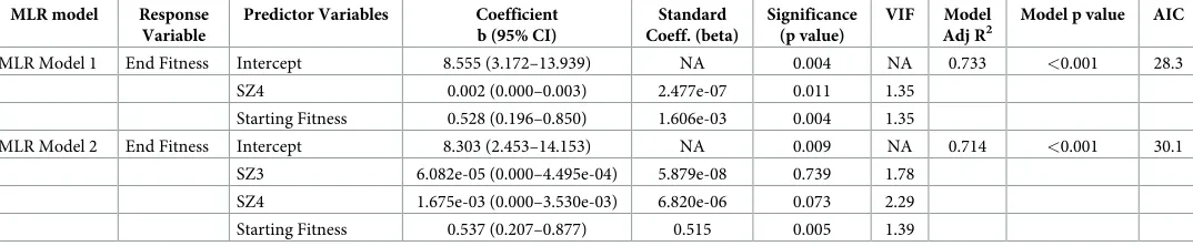
When the variables SZ3 and SZ4 were subsequently used, together with ‘starting fitness’ as

a covariate, to construct linear regression models (Table 7), it was found that the

multicolli-nearity problems disappeared, with all the VIF values being<2.5. Furthermore, the models

produced were particularly strong, both exhibiting adjusted r2values>0.7. Of the two models

produced, the one containing just the predictor variable SZ4 and ‘starting fitness’ (i.e. MLR Model 1) was the strongest, possessing an Akaike information criterion (AIC) value of 28.3 (lower than the AIC value of 30.1 for MLR Model 2, which also included variable SZ3), indicat-ing that these two variables were the most influential in predictindicat-ing end fitness, corroboratindicat-ing the results of the LOVO PLSCA.

Discussion

The overall aim of the study was to evaluate the extent to which PLSCA might be helpful when analysing TL data that exhibited considerable multicollinearity. As such, we wanted to identify

the TL variables that best related to 30-15IFTperformance in young rugby league players

fol-lowing 6-weeks of training. With respect to this, the specific findings of the current study revealed perhaps unsurprisingly, that ‘starting fitness’ is an important covariate of ‘end fitness’,

with a strong positive correlation between the two–something that others have observed [30–

31]. The strongest regression model (Table 7; MLR Model 1) suggests that professional youth

rugby league players with a lower starting fitness require a lower accumulation of distance at

very-high speed (>7 m�s-1) (compared to players with a higher starting fitness) to elicit a

Table 2. Training load (TL) data and termination speed during 30–15 intermittent fitness test for 16 professional youth rugby league players.

Player ID TD SZ1 SZ2 SZ3 SZ4 PL sRPE IndSZ PLZ1 PLZ2 PLZ3 PLZ4 Start Fitness End Fitness

1 53844 36323 14962 2196 358 7115 16027 4674 1985 3504 1269 358 16.5 18.0

2 70550 43477 22926 3682 464 8241 18848 7072 2471 4569 1051 151 16.5 17.5

3 55967 35915 16397 3376 278 5665 11952 4521 2335 2516 544 270 17.0 17.5

4 57847 35950 18612 2713 535 5798 17276 3960 2168 2806 522 270 17.0 19.0 5 42585 28529 11444 2260 352 4453 12475 3950 2001 1932 360 161 17.0 18.0

6 63157 41285 17447 3876 520 6492 15594 4712 2699 3126 530 138 17.5 19.5

7 63540 40009 18602 4227 699 6394 14806 5453 2665 2819 673 238 17.5 20.0 8 63833 41708 18462 3090 567 6955 13744 4180 2692 3484 630 150 17.5 19.0

9 47832 29853 13184 3885 897 4988 12059 4379 2145 2353 381 109 17.5 19.0

10 67531 42024 20176 4491 840 7221 15251 5152 2805 3215 845 356 18.5 19.5

11 54425 34689 16342 2911 483 5655 15039 2870 2270 2766 460 160 18.5 19.0 12 62172 39659 17703 4094 705 6072 16563 4574 2766 2670 514 123 18.5 20.0

13 76006 45183 23589 6133 1100 8041 13024 8178 2688 3776 1157 421 19.0 20.5

14 35828 21557 10290 2989 992 3524 14590 2982 1362 1601 318 242 19.0 20.5

15 52281 33999 15164 2272 633 5928 14316 3279 2204 2956 568 200 19.5 19.5 16 47583 28391 15613 3154 425 4546 11090 2919 2102 1967 378 100 19.5 20.0

Mean 57186 36159 16932 3459 616 6068 14541 4553 2335 2879 638 215 17.9 19.2

SD 10579 6491 3626 1012 240 1294 2102 1442 386 750 292 98 1.0 1.0

Abbreviations: TD = total distance (m); SZ1 = speed zone 1 (0 to 3 m�s-1; [m]); SZ2 = speed zone 2 (3.1 to 5 m�s-1; [m]); SZ3 = speed zone 3 (5.1 to 7 m�s-1; [m]); SZ4 = speed zone 1 (>7.1 m�s-1; [m]); PL = PlayerLoad (AU); PLZ1 = PlayerLoad Zone 1 (0 to 1 AU); PLZ2 = PlayerLoad Zone 2 (1.1 to 2 AU); PLZ3 = PlayerLoad Zone 3 (2.1 to 3 AU); PLZ4 = PlayerLoad Zone 4 (>3.1 AU); sRPE = session-rating-of-perceived-exertion; IndSZ = Individualised speed zone (>30–15 intermittent fitness test termination speed).

comparable incremental improvement in end fitness (e.g. +1 km�h-1in v30-15IFT) following

6-weeks of training. This model suggests, for example, that a professional youth rugby league

player with a starting v30-15IFTof 17.5 km�h-1would require an accumulation of 350m at

very-high speed over 6-weeks to improve their v30-15IFTby 1 km�h-1compared to 1050m for a

player with a starting fitness of 20.5 km�h-1. As such, this regression model could be used to

translate TL data (in conjunction with starting fitness) into practical targets for the applied practitioner working with youth rugby league players. However, it is important to note that this relationship (and associated MLR model) was observed within a single team, meaning the variability between players in the accumulated distances at very-high-speed are specific to the

context of the training modalities prescribed by the coaching staff at this club [32]. We

there-fore recommend that future researchers conduct randomised control trials with appropriate comparator arms in order to consolidate or refute our findings regarding the importance of

Table 3. Results of the Pearson correlation analysis between training load variables, starting fitness and end fitness.

TD SZ1 SZ2 SZ3 SZ4 PL sRPE IndSZ PLZ1 PLZ2 PLZ3 PLZ4 Starting

Fitness End Fitness

TD (r value) 1.000 0.979 0.965 0.683 0.157 0.925 0.403 0.796 0.875 0.841 0.666 0.342 -0.140 0.022

TD [p value] NA [0.000] [0.000] [0.004] [0.560] [0.000] [0.122] [0.000] [0.000] [0.000] [0.005] [0.195] [0.605] [0.937]

SZ1 (r value) 0.979 1.000 0.907 0.569 0.038 0.938 0.433 0.738 0.895 0.857 0.668 0.307 -0.239 -0.079

SZ1 [p value] [0.000] NA [0.000] [0.021] [0.889] [0.000] [0.094] [0.001] [0.000] [0.000] [0.005] [0.248] [0.372] [0.771]

SZ2 (r value) 0.965 0.907 1.000 0.656 0.143 0.882 0.414 0.775 0.776 0.824 0.648 0.335 -0.083 0.026

SZ2 [p value] [0.000] [0.000] NA [0.006] [0.597] [0.000] [0.111] [0.000] [0.000] [0.000] [0.007] [0.205] [0.761] [0.922]

SZ3 (r value) 0.683 0.569 0.656 1.000 0.651 0.483 -0.044 0.749 0.616 0.341 0.345 0.335 0.226 0.457

SZ3 [p value] [0.004] [0.021] [0.006] NA [0.006] [0.058] [0.872] [0.001] [0.011] [0.197] [0.191] [0.205] [0.401] [0.075]

SZ4 (r value) 0.157 0.038 0.143 0.651 1.000 0.048 -0.048 0.317 0.066 -0.017 0.065 0.309 0.511 0.738

SZ4 [p value] [0.560] [0.889] [0.597] [0.006] NA [0.860] [0.860] [0.232] [0.807] [0.951] [0.810] [0.244] [0.043] [0.001]

PL (r value) 0.925 0.938 0.882 0.483 0.048 1.000 0.487 0.792 0.722 0.965 0.858 0.418 -0.278 -0.180

PL [p value] [0.000] [0.000] [0.000] [0.058] [0.860] NA [0.056] [0.000] [0.002] [0.000] [0.000] [0.108] [0.296] [0.505]

sRPE (r value) 0.403 0.433 0.414 -0.044 -0.048 0.487 1.000 0.261 0.195 0.568 0.399 0.088 -0.347 -0.149

sRPE [p value] [0.122] [0.094] [0.111] [0.872] [0.860] [0.056] NA [0.329] [0.468] [0.022] [0.126] [0.745] [0.188] [0.582]

IndSZ (r value) 0.796 0.738 0.775 0.749 0.317 0.792 0.261 1.000 0.552 0.731 0.749 0.469 -0.264 -0.054

IndSZ [p value] [0.000] [0.001] [0.000] [0.001] [0.232] [0.000] [0.329] NA [0.027] [0.001] [0.001] [0.067] [0.323] [0.843]

PLZ1 (r value) 0.875 0.895 0.776 0.616 0.066 0.722 0.195 0.552 1.000 0.590 0.346 0.056 -0.060 0.076

PLZ1 [p value] [0.000] [0.000] [0.000] [0.011] [0.807] [0.002] [0.468] [0.027] NA [0.016] [0.190] [0.835] [0.824] [0.780]

PLZ2 (r value) 0.841 0.857 0.824 0.341 -0.017 0.965 0.568 0.731 0.590 1.000 0.828 0.301 -0.336 -0.281

PLZ2 [p value] [0.000] [0.000] [0.000] [0.197] [0.951] [0.000] [0.022] [0.001] [0.016] NA [0.000] [0.257] [0.204] [0.292]

PLZ3 (r value) 0.666 0.668 0.648 0.345 0.065 0.858 0.399 0.749 0.346 0.828 1.000 0.662 -0.280 -0.202

PLZ3 [p value] [0.005] [0.005] [0.007] [0.191] [0.810] [0.000] [0.126] [0.001] [0.190] [0.000] NA [0.005] [0.293] [0.453]

PLZ4 (r value) 0.342 0.307 0.335 0.335 0.309 0.418 0.088 0.469 0.056 0.301 0.662 1.000 -0.018 0.079

PLZ4 [p value] [0.195] [0.248] [0.205] [0.205] [0.244] [0.108] [0.745] [0.067] [0.835] [0.257] [0.005] NA [0.948] [0.771]

Starting Fitness (r value) -0.140 -0.239 -0.083 0.226 0.511 -0.278 -0.347 -0.264 -0.060 -0.336 -0.280 -0.018 1.000 0.784

Starting Fitness [p value] [0.605] [0.372] [0.761] [0.401] [0.043] [0.296] [0.188] [0.323] [0.824] [0.204] [0.293] [0.948] NA [0.000]

End Fitness (r value) 0.022 -0.079 0.026 0.457 0.738 -0.180 -0.149 -0.054 0.076 -0.281 -0.202 0.079 0.784 1.000

End Fitness [p value] [0.937] [0.771] [0.922] [0.075] [0.001] [0.505] [0.582] [0.843] [0.780] [0.292] [0.453] [0.771] [0.000] NA

Abbreviations: TD = total distance (m); SZ1 = speed zone 1 (0 to 3 m�s-1; [m]); SZ2 = speed zone 2 (3.1 to 5 m�s-1; [m]); SZ3 = speed zone 3 (5.1 to 7 m�s-1; [m]); SZ4 = speed zone 1 (>7.1 m�s-1; [m]); PL = PlayerLoad (AU); PLZ1 = PlayerLoad Zone 1 (0 to 1 AU); PLZ2 = PlayerLoad Zone 2 (1.1 to 2 AU); PLZ3 = PlayerLoad Zone 3 (2.1 to 3 AU); PLZ4 = PlayerLoad Zone 4 (>3.1 AU); sRPE = session-rating-of-perceived-exertion; IndSZ = Individualised speed zone (>30–15 intermittent fitness test termination speed).

the interaction between the distance accumulated at very-high speed and a players starting ‘fit-ness’ to improving prolonged intermittent running ability in team sport athletes.

Consistent with previous research [4–5,8–11], the findings of the current study indicate

that variables commonly used to assess TL tend to be highly correlated (Table 3) and thus

con-tain considerable shared information. As such, they violate assumptions regarding

multicolli-nearity (Table 4), which can be problematic when performing MLR analysis [13–14]. While

multicollinearity issues can be addressed by removing variables with a ‘high VIF’ value, this has the disadvantage that it is rather piecemeal and involves making subjective decisions regarding VIF exclusion criteria and the variables to be excluded. Alternatively, principal

com-ponent regression (PCR) can be used [33–34]. However, while PCR is immune to

multicolli-nearity, it has the great disadvantage that it requires the construction of composite predictor variables, which are difficult to interpret. In response to this, we developed the LOVO PLSCA methodology presented above as an alternative for analysing multicollineated data sets. The results of the current study suggest that the LOVO PLSCA strategy is well suited to the analysis of highly correlated sports performance data, suggesting that it might be a useful tool for researchers and practitioners seeking to better understand the factors that influence sports performance.

The LOVO PLSCA approach echoes that of the ‘decrease in Gini impurity’ strategy

fre-quently used with random forests to quantify variable importance [23]. As such, it represents a

new orthogonal approach for quantifying variable importance that is immune to multicolli-nearity and can be used as a variable filtering tool prior to MLR. Furthermore, unlike MLR, which struggles when the number of predictor variables exceeds the number of subjects or

observations [35]., PLSCA is not affected by this problem. With PLSCA it is possible to explore

the relationship between multiple predictor variables and multiple response variables, enabling complex relationships within the data to be evaluated–something that may be of great value when investigating broad latent constructs such as ‘strength’, ‘fatigue’ or ‘technical-tactical per-formance’. Say for example, we wanted to evaluate the relationship between, ‘fatigue’ status (measured using the variables: ‘change in countermovement jump height’; ‘perceived recov-ery’; and ‘6 second watt bike test’) and ‘physical performance’ (measured using the variables:

‘v30-15IFT’; ‘40 metre maximal sprint speed’; and ‘3 repetition maximal squat and bench

Table 4. Baseline multiple linear regression model with end fitness as the response variable, showing the calculated variable inflation factors (VIFs).

Response Variable

Predictor Variables Coefficient

(b)

Significance (p value)

VIF Model Metrics

Adj r2 (p value)

End Fitness Intercept 1.289e+01 0.426 NA 0.562 (0.324)

TD 1.322e-03 0.876 224288.3

SZ1 -8.480e-04 0.920 83232.3

SZ2 -1.172e-03 0.886 24699.2

SZ3 -1.529e-03 0.853 1930.9

SZ4 2.432e-03 0.765 104.0

PL -1.206e-03 0.985 203338.7

sRPE -3.599e-05 0.823 3.2

IndSZ -2.923e-04 0.670 26.1

PLZ1 -3.033e-03 0.962 17170.2

PLZ2 -2.006e-03 0.975 65129.4

PLZ3 4.597e-03 0.945 10600.5

PLZ4 -7.791e-03 0.905 1131.4

Starting Fitness 3.200e-01 0.691 18.0

press’). With PLSCA it would be possible to investigate the relationship between the four ‘physical performance’ variables and the three ‘fatigue’ variables, something that would be dif-ficult using a more conventional approach.

Although LOVO PLSCA can be used to assess the relative importance of predictor vari-ables, because it is not a regression technique it cannot explicitly predict the response variables

from a set of predictor variables [19]. In order to do this a related technique, partial least

squares regression (PLSR), has been developed [19,21]. While consideration of PLSR is beyond

the scope of the current paper, it is worth noting that PLSR shares many similarities with PCR

Table 5. Results of the LOVO PLSCA showing the effect on singular value inertia of omitting variables one at a time.

PLSCA Model Response variables Predictor variables

No. of subjects included

No. of simulations

Measured inertia

Change in inertia compared to baseline

Significance p value PLSCA Baseline End Fitness, Starting Fitness

TD, SZ1, SZ2, SZ3, SZ4, PL, sRPE, IndSZ, PLZ1, PLZ2, PLZ3, PLZ4

16 10000 25.096 NA 0.271

Omit TD End Fitness, Starting Fitness

SZ1, SZ2, SZ3, SZ4, PL, sRPE, IndSZ, PLZ1, PLZ2, PLZ3, PLZ4

16 10000 24.785 0.311 0.240

Omit SZ1 End Fitness, Starting Fitness

TD, SZ2, SZ3, SZ4, PL, sRPE, IndSZ, PLZ1, PLZ2, PLZ3, PLZ4

16 10000 24.512 0.584 0.253

Omit SZ2 End Fitness, Starting Fitness

TD, SZ1, SZ3, SZ4, PL, sRPE, IndSZ, PLZ1, PLZ2, PLZ3, PLZ4

16 10000 24.967 0.129 0.232

Omit SZ3 End Fitness, Starting Fitness

TD, SZ1, SZ2, SZ4, PL, sRPE, IndSZ, PLZ1, PLZ2, PLZ3, PLZ4

16 10000 23.151 1.945 0.774

Omit SZ4 End Fitness, Starting Fitness

TD, SZ1, SZ2, SZ3, PL, sRPE, IndSZ, PLZ1, PLZ2, PLZ3, PLZ4

16 10000 19.170 5.926 0.547

Omit PL End Fitness, Starting Fitness

TD, SZ1, SZ2, SZ3, SZ4, sRPE, IndSZ, PLZ1, PLZ2, PLZ3, PLZ4

16 10000 24.352 0.744 0.261

Omit sRPE End Fitness, Starting Fitness

TD, SZ1, SZ2, SZ3, SZ4, PL, IndSZ, PLZ1, PLZ2, PLZ3, PLZ4

16 10000 23.897 1.200 0.273

Omit IndSZ

End Fitness, Starting Fitness

TD, SZ1, SZ2, SZ3, SZ4, PL, sRPE, PLZ1, PLZ2, PLZ3, PLZ4

16 10000 24.308 0.788 0.260

Omit PLZ1 End Fitness, Starting Fitness

TD, SZ1, SZ2, SZ3, SZ4, PL, sRPE, IndSZ, PLZ2, PLZ3, PLZ4, Starting Fitness

16 10000 24.913 0.183 0.233

Omit PLZ2 End Fitness, Starting Fitness

TD, SZ1, SZ2, SZ3, SZ4, PL, sRPE, IndSZ, PLZ1, PLZ3, PLZ4

16 10000 23.906 1.190 0.278

Omit PLZ3 End Fitness, Starting Fitness

TD, SZ1, SZ2, SZ3, SZ4, PL, sRPE, IndSZ, PLZ1, PLZ2, PLZ4

16 10000 24.325 0.771 0.258

Omit PLZ4 End Fitness, Starting Fitness

TD, SZ1, SZ2, SZ3, SZ4, PL, sRPE, IndSZ, PLZ1, PLZ2, PLZ3

16 10000 24.996 0.100 0.224

Abbreviations: TD = total distance (m); SZ1 = speed zone 1 (0 to 3 m�s-1_{; [m]); SZ2 = speed zone 2 (3.1 to 5 m�s}-1_{; [m]); SZ3 = speed zone 3 (5.1 to 7 m�s}-1_{; [m]);}

SZ4 = speed zone 1 (>7.1 m�s-1_{; [m]); PL = PlayerLoad (AU); PLZ1 = PlayerLoad Zone 1 (0 to 1 AU); PLZ2 = PlayerLoad Zone 2 (1.1 to 2 AU); PLZ3 = PlayerLoad}

Zone 3 (2.1 to 3 AU); PLZ4 = PlayerLoad Zone 4 (>3.1 AU); sRPE = session-rating-of-perceived-exertion; IndSZ = Individualised speed zone (>30–15 intermittent fitness test termination speed).

in so much that both techniques are primarily used for prediction and require the construction of composite predictor variables, albeit using different methodologies. As such, PLSR suffers from the same drawback as PCR, namely that the models produced are difficult to interpret because the predictors are not the original measured variables. By comparison, PLSCA, when used as a filtering tool and combined with MLR, overcomes any multicollinearity problems and is much easier to interpret.

Conclusions

The findings of the current study demonstrate that multicollinearity is a major limiting factor, which has the potential to compromise analysis of TL data. However, this problem can be

Fig 2. Variable importance plot showing the decrease in singular value inertia attributable to each predictor variable.

overcome by using an orthogonal PLSCA approach, which is immune to multicollinearity, thus enabling the user to quantify the strength of the relationships between the respective vari-ables. Using LOVO PLSCA we were able to identify those variables that were most influential in explaining improvements in player fitness. This enabled us to remove irrelevant variables and so overcome any multicollinearity issues. This allowed us to produce a robust MLR model for predicting ‘end fitness’, from which we inferred that ‘starting fitness’ and the accumulation of distance at ‘very-high speed’ across a 6-week period of training were the most influential predictors of end fitness in professional youth rugby league players. As such, PLSCA appears to be a useful tool for filtering out irrelevant information and identifying those variables that should be included prior to any given MLR analysis.

Acknowledgments

The authors would like to thank Professor Charles Taylor (University of Leeds) for his helpful suggestions regarding the PLSCA methodology and Melissa Bargh for her assistance in the data collection.

Author Contributions

Conceptualization: Dan Weaving, Clive B. Beggs.

Table 6. Results of the PLSCA using refined models.

PLSCA model

Response variables

Predictor variables

No. of subjects included

No. of simulations

Measure inertia

Significance p value

Chi-square (p values) [Cramers

V]

PLSCA Baseline

End Fitness, Starting Fitness

TD, SZ1, SZ2, SZ3, SZ4, PL, sRPE, IndSZ, PLZ1, PLZ2, PLZ3, PLZ4

16 10000 25.096 0.271 NA

PLSCA Model 1

End Fitness, Starting Fitness

SZ4 16 10000 13.459 0.007� _709.5

(<0.0001) [0.188] PLSCA

Model 2

End Fitness, Starting Fitness

SZ3, SZ4 16 10000 16.419 0.015� _2030.8

(<0.0001) [0.319]

Abbreviations: TD = total distance (m); SZ1 = speed zone 1 (0 to 3 m�s-1; [m]); SZ2 = speed zone 2 (3.1 to 5 m�s-1; [m]); SZ3 = speed zone 3 (5.1 to 7 m�s-1; [m]); SZ4 = speed zone 1 (>7.1 m�s-1; [m]); PL = PlayerLoad (AU); PLZ1 = PlayerLoad Zone 1 (0 to 1 AU); PLZ2 = PlayerLoad Zone 2 (1.1 to 2 AU); PLZ3 = PlayerLoad Zone 3 (2.1 to 3 AU); PLZ4 = PlayerLoad Zone 4 (>3.1 AU); sRPE = session-rating-of-perceived-exertion; IndSZ = Individualised speed zone (>30–15 intermittent fitness test termination speed).

�_{p values less than 0.05 considered significant for one-tailed test}

https://doi.org/10.1371/journal.pone.0211776.t006

Table 7. Results of refined MLR models with respective variable inflation factors.

MLR model Response

Variable

Predictor Variables Coefficient

b (95% CI)

Standard Coeff. (beta)

Significance (p value)

VIF Model

Adj R2

Model p value AIC

MLR Model 1 End Fitness Intercept 8.555 (3.172–13.939) NA 0.004 NA 0.733 <0.001 28.3

SZ4 0.002 (0.000–0.003) 2.477e-07 0.011 1.35 Starting Fitness 0.528 (0.196–0.850) 1.606e-03 0.004 1.35

MLR Model 2 End Fitness Intercept 8.303 (2.453–14.153) NA 0.009 NA 0.714 <0.001 30.1

SZ3 6.082e-05 (0.000–4.495e-04) 5.879e-08 0.739 1.78

SZ4 1.675e-03 (0.000–3.530e-03) 6.820e-06 0.073 2.29 Starting Fitness 0.537 (0.207–0.877) 0.515 0.005 1.39

Data curation: Matt Ireton, Sarah Whitehead.

Formal analysis: Dan Weaving, Clive B. Beggs.

Funding acquisition: Ben Jones.

Methodology: Dan Weaving, Sarah Whitehead, Clive B. Beggs.

Project administration: Dan Weaving, Kevin Till.

Supervision: Ben Jones, Kevin Till, Clive B. Beggs.

Writing – original draft: Dan Weaving, Kevin Till, Clive B. Beggs.

Writing – review & editing: Dan Weaving, Ben Jones, Matt Ireton, Sarah Whitehead, Kevin Till, Clive B. Beggs.

References

1. Cardinale M & Varley MC. Wearable training-monitoring technology: applications, challenges and opportunities. Int J Sports Physiol Perform. 2017; 12: S255–S262. https://doi.org/10.1123/ijspp.2016-0423PMID:27834559

2. Graham MH. Confronting multicollinearity in ecological multiple regression. Ecology. 2003; 84(11): 2809–2815.

3. Slinker BK & Glantz SA. (1985). Multiple regression for physiological data analysis: the problem of multi-collinearity. Am J Physiol. 1985; 249(1 Pt 2): R1–12.https://doi.org/10.1152/ajpregu.1985.249.1.R1 PMID:4014489

4. Weaving D, Marshall P, Earle K, Nevill A & Abt G. Combining internal- and external-training-load mea-sures in professional rugby league. Int J Sports Physiol Perform. 2014; 9: 905–912.https://doi.org/10. 1123/ijspp.2013-0444PMID:24589469

5. McLaren SJ, Macpherson TW, Coutts AJ, Hurst C, Spears IR & Weston M. The relationships between internal and external measures of training load and intensity in team sports: a meta-analysis. Sports Med. 2018; 48(3): 641–658.https://doi.org/10.1007/s40279-017-0830-zPMID:29288436

6. Woods CT, Sinclair W & Robertson S. Explaining match outcome and ladder position in the National Rugby League using team performance indicators. J Sci Med Sport. 2017; 20(12): S1440–2440. 7. Hulin BT, Gabbett TJ, Lawson DW, Caputi P & Sampson JA. The acute:chronic workload ratio predicts

injury: high chronic workload may decrease injury risk in elite rugby league players. Br J Sports Med. 2016; 50(4): 231–236.https://doi.org/10.1136/bjsports-2015-094817PMID:26511006

8. Oxendale CL, Twist C, Daniels M & Highton J. The relationship between match-play characteristics of elite rugby league and indirect markers of muscle damage. Int J Sports Physiol Perform. 2016; 11: 515– 521.https://doi.org/10.1123/ijspp.2015-0406PMID:26355239

9. Akubat I, Patel E, Barrett S, & Abt G. Methods of monitoring the training and match load and their rela-tionship to changes in fitness in professional youth soccer players. J Sports Sci. 2012; 30: 1473–1480. https://doi.org/10.1080/02640414.2012.712711PMID:22857397

10. Taylor R, Sanders D, Myers T, Abt G, Taylor CA & Akubat I. The dose-response relationship between training load and aerobic fitness in academy rugby union players. Int J Sports Physiol Perform. 2017; 22: 1–22.

11. Weaving D, Jones B, Marshall P, Till K & Abt G. Multiple measures are needed to quantify training loads in professional rugby league. Int J Sports Med. 2017; 38: 735–740. https://doi.org/10.1055/s-0043-114007PMID:28783849

12. Weaving D, Jones B, Till K, Abt G, Beggs C. The case for adopting a multivariate approach to optimise training load quantification in team sports. Front Physiol. 2017; 8: 1024.https://doi.org/10.3389/fphys. 2017.01024PMID:29311959

13. Marquardt DW. Generalized inverses, ridge regression, biased linear estimation, and nonlinear estima-tion. Technometrics. 1970; 12: 591–256.

14. Mason RL, Gunst RF & Hess JL. Statistical design and analysis of experiments: applications to engi-neering and science. New York: Wiley; 1989.

16. Golub GH & Kahan W. Calculating the singular values and pseudo-inverse of a matrix. SIAM J Appl Math Series B, Numerical Analysis.1965; 2(2): 205–224.

17. McIntosh AR, Misic B. Multivariate statistical analyses for neuroimaging data. Annu Rev Psychol. 2013; 64: 499–525.https://doi.org/10.1146/annurev-psych-113011-143804PMID:22804773

18. Till K, Jones BL, Cobley S, Morley D, O’Hara J, Chapman C et al. Identifying Talent in Youth Sport: A Novel Methodology Using Higher-Dimensional Analysis. PLoS One. 2016; 11(5):e0155047.https://doi. org/10.1371/journal.pone.0155047PMID:27224653

19. Krishnan A, Williams LJ, McIntosh AR & Abdi H. Partial Least Squares (PLS) methods for neuroimag-ing: a tutorial and review. Neuroimage. 2011; 56(2): 455–75.https://doi.org/10.1016/j.neuroimage. 2010.07.034PMID:20656037

20. Levine B, Kovacevic N, Nica EI, Schwartz ML, Gao F & Black SE. Quantified MRI and cognition in TBI with diffuse and focal damage. Neuroimage Clin. 2013; 2: 534–541.https://doi.org/10.1016/j.nicl.2013. 03.015PMID:24049744

21. Abdi H & Williams LJ. Partial least squares methods: partial least squares correlation and partial least square regression. Methods Mol Biol. 2013; 930: 549–579. https://doi.org/10.1007/978-1-62703-059-5_23PMID:23086857

22. Beggs CB, Magnano C, Belov P, Krawiecki J, Ramasamy DP Hagemeier J et al. Internal Jugular Vein Cross-Sectional Area and Cerebrospinal Fluid Pulsatility in the Aqueduct of Sylvius: A Comparative Study between Healthy Subjects and Multiple Sclerosis Patients. PLoS One. 2016; 11(5): e0153960. https://doi.org/10.1371/journal.pone.0153960PMID:27135831

23. Louppe G, Wehenkel L, Sutera A & Geurts P. Understanding variable importances in forests of random-ized trees. Neural Information Processing Systems Conference: Advances in Neural Information Pro-cessing Systems. 2013; 26.

24. Darrall-Jones JD, Jones B & Till K. The effect of body mass on the 30–15 intermittent fitness test in rugby union players. Int J Sports Physiol Perform. 2016; 11(3): 400–403.https://doi.org/10.1123/ijspp. 2015-0231PMID:26217047

25. Malone JJ, Lovell R, Varley MC & Coutts AJ. Unpacking the black box: applications and considerations for using GPS devices in sport. Int J Sports Physiol Perform. 2017; 12(Suppl 2): S218–S226.https://doi. org/10.1123/ijspp.2016-0236PMID:27736244

26. Varley MC, Jaspers A, Helsen WF & Malone JJ. Methodological considerations when quantifying high-intensity efforts in team sport using global positioning system technology. Int J Sports Physiol Perform. 2017; 4;1–25.

27. Boyd LJ, Ball K & Aughey RJ. The reliability of MinimaxX accelerometers for measuring physical activity in Australian football. Int J Sports Physiol Perform. 2011; 6(3): 311–21. PMID:21911857

28. Foster C, Florhaugh JA, Franklin J, Gottschall L, Hrovatin LA, Parker S, et al. A new approach to moni-toring exercise training. J Strength Cond Res. 2001; 15: 109–115. PMID:11708692

29. Allison PD. Change Scores as Dependent Variables in Regression Analysis. Sociological Methodology. 1990; 20; 93–114

30. Skinner JS, Jasko´lski A, Jasko´ lski A, Krasnoff J, Gagnon J, Leon AS, et al. Age, sex, race, initial fitness, and response to training: the HERITAGE Family Study. J Appl Physiol. 1985; 90:1770–1776.

31. Astorino TA, Schubert MM. Individual responses to completition of short-term and chronic interval train-ing: a retrospective study. PLoS One. 2014; 21:e97638.

32. Weaving D, Jones B, Till K, Marshall P, Earle K, Abt G. Quantifying the external and internal loads of professional rugby league training modes: consideration for concurrent field-based training prescription. J Strength Cond Res. 2017;https://doi.org/10.1519/JSC.0000000000002242PMID:28930869 33. Minitab blog editor. Enough Is Enough! Handling Multicollinearity in Regression Analysis. 16th April

2013. http://blog.minitab.com/blog/understanding-statistics/handling-multicollinearity-in-regression-analysis(accessed 6th May 2018)

34. James G, Witten D, Hastie T & Tibshirani R. An introduction to statistical learning with applications in R. Springer texts in statistics. Springer, New York; 2013.