Linear Quadratic Gaussian (LQG) controller for inverted pendulum

LINEAR QUADRATIC GAUSSIAN (LQG) CONTROLLER FOR INVERTED PENDULUM

NORHIDAYAH BINTI AHMAD

A project report submitted in partial fulfillment of the requirement for the award of the Degree

Master of Electrical Engineering

Faculty of Electrical and Electronic Engineering University Tun Hussein Onn Malaysia

ABSTRACT

ABSTRAK

CONTENTS

TITLE i

DECLARATION ii

DEDICATION iii

ACKNOLEDGEMENT iv

ABSTRACT v

ABSTRAK vi

TABLE OF CONTENTS vii

LIST OF TABLES x

LIST OF FIGURES xi

LIST OF SYMBOL AND ABBREVIATIONS xiii

LIST OF APPENDICES xiv

CHAPTER 1 INTRODUCTION 1.1 Overview 1 1.2 Problem Statement 2 1.3 Objectives of the project 2 1.4 Project Scope 3

1.5 Thesis outline 3

CHAPTER 2 LITERATURE REVIEW 2.1 Introduction 5

2.2 Inverted pendulum system 5 2.2.1 Mathematical model of inverted pendulum system 8

2.3 Control theory 11

2.3.1 Linear quadratic optimal 11

2.3.3 Observability and controllability 15

2.3.4 Kalman filter 16

2.4 System response 17

2.5 Matrix Laboratory software 18

2.6 Microcontroller Arduino Mega 2560 19

2.7 The motor and control circuit 20

2.8 Feedback device 21

2.9 Previous case study 23

CHAPTER 3 METHODOLOGY 3.1 Introduction 26

3.2 Design overview 26

3.3 Mathematical model 28

3.3.1 Inverted pendulum mathematical model 28

3.3.2 Linear quadratic optimal mathematical model 42

3.3.3 Optimal state estimation 44

3.4 Procedure for software approach 50

3.5 Hardware 53

3.5.1 DC gear motor with encoder 53

3.5.2 Analog rotary position sensor 55

CHAPTER 4 RESULT AND ANALYSIS 4.1 Introduction 58

4.2 Inverted pendulum system mathematical model 58

4.2.1 State Space Equation 58

4.2.2 Continuous transfer function 60

4.2.3 Discrete transfer function 60

4.3 Controllability and observability of the system 62

4.4 Inverted pendulum without controller 63

4.5 Optimal Linear Quadratic 65

4.6 Kalman state estimation gain 66

4.7 Steady state LQG controller 66

4.8 Closed loop analysis 67

4.9.1 Speed of the motor 70 4.8.2 Encoder direction 71 4.8.3 Angle position 74

CHAPTER 5 CONCLUSION

5.1 Conclusion 76

5.2 Recommendations 77

REFERENCES 78

APPENDIX A: Simulation 81

APPENDIX B: Encoder direction 84

APPENDIX C: Reading the sensor value 85

LIST OF TABLES

2.1 Parameter Description in Inverted Pendulum System 9

3.1 Parameter in Inverted Pendulum System 37

4.1 Poles and zeros location for open loop system 63

4.2 Matrix Riccati Equation for 4 phases 64

4.3 Performance Indices for Control System 67 4.4 Poles and zeros location for open loop system 68 4.5 Table of Voltage and Speed of Motor 69

4.6 Encoder sequence for clockwise 71

4.7 Encoder sequence for anti-clockwise 71

LIST OF FIGURES

2.1 Overview Inverted Pendulum System 6

2.2 A Single Pendulum Type 6

2.3 A Double Pendulum Type 7

2.4 Mobile Inverted Pendulum Type 7

2.5 A Rotary Inverted Pendulum Type 7

2.6 Free Body Diagram of Inverted Pendulum 8 2.7 Block Diagram of Discrete-Time Control System 10

2.8 State Space System with Feedback 13

2.9 Observer-State Feedback Control System 14

2.10 Kalman Filter Predictor-Corrector 17

2.11 Transient Response Specification 18

2.12 Pin Description Mega2560 20

2.13 Parts in DC Motor 21

2.14 Encoder Parts 22

3.1 Flow Chart of Project Procedure 27

3.2 Force Applied to Cart 29

3.3 Observer Block Diagram 46

3.4 LQG Block Diagram 48

3.5 Digital Controller System 48

3.6 Simulink for System without Controller 50

3.7 Control System in Simulink 52

3.8 DC Motor SPG30K-20 54

3.9 Connection between Arduino and Motor 54

3.10 Connection for Encoder Test 54

3.12 Connection for Testing Sensor 55

3.13 Movement of Angle Sign 56

4.1 System without Controller 62

4.2 Poles Location of Position System 63

4.3 Control System for Closed Loop System 66 4.4 Response Specification of Closed Loop System 66 4.5 Poles and Zeros Location for Control System 68

4.6 Speed versus Voltage Graph 70

4.7 Encoder Pulses when Motor+ connect to Power Supply 71 4.8 Analysis Encoder Pulses according Phase for Figure 4.7 72 4.9 Decoder Pulses when Motor+ Connect to Ground 72 4.10 Analysis of Decoder Pulses from Figure 4.9 73

LIST OF SYMBOL AND ABBREVIATIONS

- Mass of the cart - Mass of the Pendulum

- Angular Acceleration of the Pendulum

- Length of pendulum

- Moment of inertia of the pendulum

- Position of the cart ̇ - Velocity of the Cart ̈ - Acceleration of the Cart

- Pendulum Angle or Angular Displacement ̇ - Angular Velocity of the Pendulum

̈ - Angular Acceleration of the Pendulum , - Weighting control

- Steady state Riccati equation for feedback gain - State feedback gain

, - covariance matrix

- Steady state Riccati equation for Kalman gain

- Kalman gain

LIST OF APPENDICES

APPENDIX TITLE

A Simulation 81

B Encoder direction 84

C Reading the sensor value 85

D Gantt chart for Master Project 1 (PS 1) 86

CHAPTER 1

INTRODUCTION

1.1Overview

The inverted pendulum system is popular and widely used as a benchmark for testing control algorithms area. The system is nonlinear, unstable systems which showcase modern control methods.

The concept of inverted pendulum can visualize through relationship between hand and broom stick. When the broom stick need to balance by hand, the position of hand need to constantly adjust to make sure the broom-stick not fall down. The limitation of this visualize compare to the inverted pendulum system is by control with hand, the hand can move freely while the built inverted pendulum system can only move in one dimension.

An ideal controller is the controller would keep the pendulum in upright condition with little change in the angle of the pendulum or the cart displacement. But limitations would be imposed based on the actual parameter of the system. Therefore, designing controller that is close to ideal is challenging design problem.

1.2 Problem Statement

Inverted pendulum is a free hung pendulum which is upright and base on ground and it naturally fall downward due to gravity. This is show that the inverted pendulum is inherently unstable system. The inverted pendulum system is combination of linear system (position of cart) and oscillatory dynamic (angle of pendulum).

Practically, in system there must be some noise and other inaccuracies either in plant or in sensor measurement, this inaccuracies and noise can affect the performance of the system. Inverted pendulum system also undergoes this problem. Because of this, with help appropriate controller can reduce the inaccuracies and noise toward the system.

Since inverted pendulum system is unstable and undergoes noise and inaccuracies in the system, in order to stabilize and eliminate the noises in the inverted pendulum, Linear Quadratic Gaussian (LQG) has been studied. LQG are combination of multivariate feedback such as Linear Quadratic Regulator (LQR) with Kalman Filter. Kalman filter is used to estimate the unmeasured variable and to filter those that are directly measured. Then LQR feedback strategy is then used to stabilize the system. Hopefully, with implemented LQG controller in inverted pendulum, the system can be stable.

1.3 Objectives of the project

The objectives of this project are:

1.4 Project scope

The scopes ranges that will be cover in this project are:

i. Design and implemented the mathematical model of inverted pendulum system. ii. Obtain optimal linear quadratic controller gain for a system by using Ricatti

equation.

iii. Implement concept of Kalman filter in system and to design Linear Quadratic Gaussian controller.

iv. The design of the system and controller was implemented through Matlab software.

v. Manipulate the control weighting and noise covariance matrix properly to gain better state feedback gain and Kalman gain to give better performance of the system.

1.5 Thesis outline

This thesis consists of five chapters that will explain in more details regarding this project. The first chapter will put in plain words about project overview which are about the project background, problem statement, objectives of the project and scopes of the project.

The second chapter will review about various controllers designed for the inverted pendulum system. In this chapter, the information about the controller and the inverted pendulum system available around the world are gathered. In additional, the previous studies that related to project were use as reference of the project.

The fourth chapter will discuss about the result gathered from the project. In addition, the result will be analyzed and the way of solving the problems occurred during this project will be presented.

CHAPTER 2

LITERATURE REVIEW

2.1 Introduction

Conducting the literature review is done prior to undertaking the project. Thus, as much information as needed on the technology available and methodologies used by other research counterparts around the world on the related topic are gathered. It shows that previous related studies are important as a reference of the project.

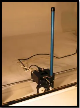
2.2 Inverted pendulum system

Figure 2. 1: Overview Inverted Pendulum System.

In general, the inverted pendulum system has several types, e.g. a single pendulum, a double pendulum, mobile pendulum, swing up pendulum, etc. Each type has different approach to balance the pendulum.

Figure 2. 3: A Double Pendulum Type.

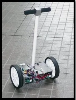
Figure 2. 4: Mobile Inverted Pendulum Type.

Since the inverted pendulum is in upright situation, is naturally easily to fall downward because of gravity. Thus the inverted pendulum system is inherently unstable. In 2-Dimensional system, to stabilize the system it can be done either vertical or horizontal oscillation with certain frequency. While for 3-Dimensional, a rotational arms or free robot arms are used. An addition, for algorithm a controller using feedback system is used to keep the pendulum upright [4, 5]. In order to make sure the inverted pendulum in stable condition, any small changes of horizontal position, ∆x in x will resulting to small adjustment of angular position, ∆θ in θ is requires so that the pendulum is always erected in its inverted position during any changes has made [7].

2.2.1 Mathematical model of inverted pendulum system

Mathematical descriptions of the inverted pendulum need to derive in order to be able to stimulate the dynamic behaviour of the system [8]. The mathematical model construction is dividing by two parts; there are the cart of pendulum and the pendulum.

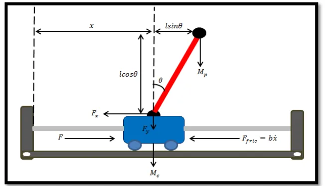
The system dynamic equation can be derived by using Newtonian method or Euler-Lagrange method. The Newtonian methods is using free body diagram while the Euler-Lagrange method is defined as the difference between potential and kinetic energy [13].

By applying the law of dynamic on the inverted pendulum system, the equation of motion are:

( ) ̈ ̇ ̈ ̈ (2.1)

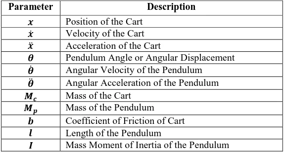
̈ ̈ ⁄ (2.2)

where is the position of the cart, is the pendulum angle or angular displacement, where the pendulum angle measured from the upright position and is force that applied to cart. In the interest of understanding, Table 2.1 is summarization of the all parameter definition in the equation motion of inverted pendulum.

Table 2. 1: Parameter Description in Inverted Pendulum System.

Parameter Description

Position of the Cart

̇ Velocity of the Cart

̈ Acceleration of the Cart

Pendulum Angle or Angular Displacement

̇ Angular Velocity of the Pendulum

̈ Angular Acceleration of the Pendulum Mass of the Cart

Mass of the Pendulum Coefficient of Friction of Cart Length of the Pendulum

Mass Moment of Inertia of the Pendulum

Since the angle or angular displacement of pendulum, which is the angle, was measured from the vertical line to pendulum, gain small value of angle refer to Figure 2.6, the small-angle approximation to inverted pendulum was applied [15].

The small-angle approximation is a simplification of the basic trigonometry function which is approximately true in the limit where the angle approaches zero and the this approximation can be applied only when a small angle is define The small-angle approximation is truncation of the Taylor series for the basic trigonometry functions to a second order approximation. The small angle approximation is:

(2.3)

(2.5)

This assumption of small angle leads to the linearized equation motion of inverted pendulum and due to linearization, the linear time invariant state space model of the system was derived according to equation (2.6).

̇

(2.6)

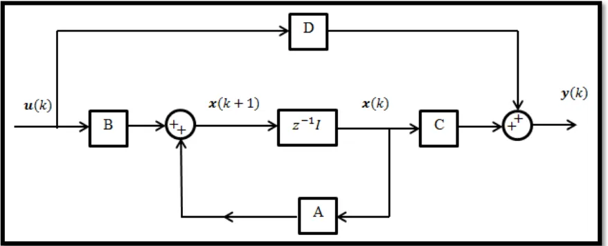
Where A with n x n matrix, B with n x r matrix, C with m x n matrix and D with m x r matrix where this matrices need for control design of the system, while u is input applied to the system and x is the state variable of the dynamic system where this variables making up the smallest set of variable determine the state of the dynamic system [15,17]. The state space method is based on system equation in term of n differential equation. The vector-matrix notation is simplification of the mathematical model of the system. The state space approach also enable the engineer to design control system with respect to given performance index and also can include the initial condition in the design. Figure 2.7 show the block diagram for discrete time control system for state space approach.

For inverted pendulum system, the state variables are ̇ ̇ . The general state space equation for inverted pendulum system is:

[ ̇ ̈ ̇ ̈ ] [ ( ) ] [ ̇ ̇ ] [ ( ) ] [ ] [ ̇ ̇

] [ ] (2.7)

2.3 Control Theory

The inverted pendulum is an unstable and nonlinear system. In order to make the pendulum in upright position where the system will be stable, the suitable controller algorithm has to be implemented.

There are several algorithm controllers that can control the inverted pendulum. The algorithm can be divided into two main groups, the conventional controller and the artificial intelligence controller. Under conventional controller are Proportional Integral Derivative (PID) and Linear Quadratic Regulator (LQR)/ Linear Quadratic Gaussian (LQG) while for Artificial Intelligence Controller, there are Fuzzy Logic Controller and Artificial Neural Network Controller.

2.3.1 Linear quadratic optimal

Linear quadratic optimal control is technique that yields the best control system. This technique is assumed that the mathematical function which is called the cost function or performance index can be written. The term optimal means that the procedure of this

minimized by trial and error method. The general form of performance index equation[18]:

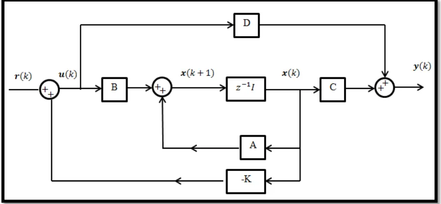
∑ (2.8) In the equation above, is the sample instant and is the terminal sample instant. Where matrix is a positive semi definite and matrix is a positive definite matrix. The matrices and determine the relative importance of the error. Then the element of feedback, are obtain to minimize the performance index. The control law of feedback is according to figure (2.8):

(2.9)

where the matrix is r x n matrix. In order to obtain the feedback gain, to make the controller optimal, the steady state solution of the Riccati equation. The Riccati equation and the feedback gain can be written as:

(2.10) (2.11)

Figure 2. 8: State Space System with Feedback

2.3.2 State estimation

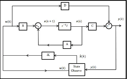
Figure 2. 9: Observer-State Feedback Control System.

State estimation is need in case the system dynamic suffers from noise. At the system output, noises always exist, by using sensor the value of noise can be measure. Since there are noise in dynamic system, the real output and the output from the model will have a difference. If is the measured output and is the measurement noise the following relation holds:

(2.12)

So, the observer can be stated as the original state description of the system with the difference that the state vector has been provided with a hat symbol. The equation above shows that the state is estimated.

From the observer state feedback control system, controller estimator transfer function can be obtained. Equation above show the controller estimator transfer function [20].

(2.14)

2.3.3 Observability and controllability

The concept of observability and controllability was introduced by R.E Kalman. This concept play important role in multivariable systems. The condition of this concept in fact, may manage the existence of a complete solution to an optimal control problem.

The observability is beneficial to solve solution regarding to unmeasured state variables. Observability is concern problem regarding of determining the state of dynamic system from observation of the output and control vector in a limited number of sampling time. The dynamic system said to be observable if, with the system in state , it is possible to determine this state from observation of the output and control vector in a limited number of sampling time [15,18,25]. For a completely observable system, given matrix

[

] (2.15)

(2.16)

Where matrix A with n x n matrix and matrix C with m x n be of rank n. The rank matrix and the conjugate transpose of the matrix give same answer.

_(2.17)

(2.18)

Where dimension of matrix A is n x n matrix and matrix B is n x r matrix is rank of by getting from row of matrix . Other way to test the completeness of the rank of square matrices is to find their determinant. The value of determinant must not equal to zero, in order to conclude the system is observable or controllable.

2.3.4 Kalman filter

Kalman filter is one of the state estimation that can estimate the state variable with the measurement include noise. If the noise is Gaussian distributed, an optimal estimator that minimizes the variance of the estimation error can be derived.

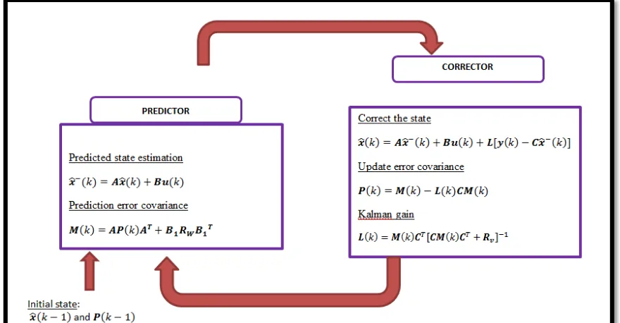
Kalman Filter is a set of mathematical equation that provides an efficient computational means to estimate the state of a process, in a way that minimizes the mean of the squared error. The Kalman filter estimates a process by using a form of feedback control: the filter estimates the process state at some time and then obtains feedback in the form of (noisy) measurements.

Figure 2. 10: Kalman Filter Predictor-Corrector 2.4 System response

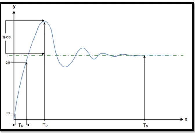
Figure 2. 11: Transient Response Specification.

From transient response specification in figure 2.11 symbol of , , are rise time, peak time and settling time respectively. The rise time is the time required for the response to rise from 10% to 90% of its final value depending on situation. Peak time is the time for the response reach the first peak of the overshoot or undershoots. While the settling time is the time required for the response curve to reach and stay within a range about the final value of a size specified as an absolute percentage of the final value usually 2%.

2.5 Matrix Laboratory software.

In MATLAB software, for modeling, simulating and analyzing dynamic systems it is easier by using Simulink approach. Simulink support linear and nonlinear system and systems can also be multirate, that is, the system can have different parts that are sampled or updated at different rates. In Simulink, the software was embedded built-in support for prototyping, testing and running models on low-cost target hardware such as Arduino.

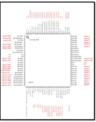
2.6 Microcontroller Arduino Mega 2560

Arduino is a single board microcontroller that usually used in electronic area for hardware project accessible. There are several type of Arduino microcontroller such as serial Arduino, Arduino Extreme, Arduino Diecimilia and many more. Chosen the type of Arduino is depending on the application of the project because different type of Arduino board give with different structure and application.

Arduino board programs are written in C or C++. The Arduino integrated development environment (IDE) comes with a software library called wiring which is it came from the original wiring project. In the programs, user only need to define two functions to make runnable cyclic executive program, that are setup() and loop() which is setup() is a function run at the start of a program. This command is to initialize setting. For loop() is a function called repeatedly. The board will run the program nonstop but once the power of the board will stop called the program.

Figure 2. 12: Pin Description Mega2560

2.7 The motor and control circuit

Figure 2. 13: Parts in DC Motor.

Figure above show the DC motor parts. When power was supply to DC motor, the electron flow from negative symbol of power supply to positive sign of power supply. Affected by the electron flow in circuit, the armature will rotate whether in clockwise or counter clockwise and resulting to movement in motor.

Second types of motor are stepper motor. The stepper motor is a brushless, synchronous electric motor that converts digital pulses into mechanical shaft rotation. The stepper motor can only take one step at a time and each step is the same size. Since each pulse causes the motor to rotate a precise angle, hence the motor position can be control without any controller.

The third types are servo motor. Mostly servo motors are used in radio-controlled model airplane, cars, boats and helicopters to control the position of wing flaps and similar devices. Servo motor is geared dc motor with a positional feedback control that allows the rotor to be positioned accurately.

2.8 Feedback device

and cumulative error associated with the transmission and feedback device to make sure the error is acceptable. In chosen the feedback device or sensor, there are several criteria need to consider. First, the application of the sensor is suitable or not for the project. Second consideration is the type of technology used in the device. For example in semiconductor manufacturing, the sensors need to be very precise in a particular environment to meet high production. The third consideration is geometry. Motion system are either linear, rotational or a combination of both motion.

There is numerous type of feedback device according to the area of application like electric current, vibration and many more. Encoder is one type sensor from electric area. Encoder is categories by three basic categories, that is motion of sensor either rotary or linear, incremental or absolute and by the method of signal generate either optical, magnetic or contacting. Encoder is a device or circuit that converts information from one format to other. Incremental encoder has simple disc pattern which this disk will interrupt light source and phototransistor this process resulting to pulses output. Then the pulses are then fed to counter, where the pulses are count in order to give position information.

Figure 2. 14: Encoder Parts.

phototransistor captured the code, encoder will send a known number of signals given angular displacement. By counting the number of signal receive in a given length of time,dt so velocity can be calculated. If the encoder rotate fast, mean the time taken is smaller this resulting to higher effectiveness of the controller.

A rotary encoder which also called shaft encoder is an electric-mechanical device that converts the angular position or motion of a shaft to an analog or digital code. Typically the application of this sensor include temperature control, speed control, position sensing, menu selection and volume control. The rotary encoder can be magnetic, optical or mechanical rotary encoder.

2.9 Previous case study

Title of project: LQG control design for balancing an inverted pendulum mobile robot Author: Ragnar Eide, Per Magne Egelid, Alexander Stamso, Hamid Reza Karimi

Title: Autonomous balancing robot design and construction of a balancing robot. Author: Christian Sundin and Filip Thorstensson

Synopsis: Purpose of this paper is to design and build a two wheeled upright robot. The robot was embedded with sensors, in order to the robot interact with surrounding the distance sensor in combination with temperature sensor was implemented on it. The robot also has a bowl on top for carrying load purpose. The controller that used to balance the robot is PID controller and linear quadratic Gaussian (LQG) controller. For testing the sensor fusion between the accelerometer and gyro, the Kalman filter and complementary filter was used. As result, Kalman filter was chosen because Kalman filter sufficient for both linear movement and noise of the accelerometer as well as estimate and compensate for the gyros drift and bias. In this project, the microcontroller has been used is Arduino Mega35. Unfortunately, the LQG controller cannot be implementing in hardware this is because Arduino is not fast enough to do calculation for the controller in the required loop time. As result, PID controller was used to balance the robot and it was successful.

Title: Modelling and control design for inverted pendulum

Author: Mr Pankaj Kumar, Mr. Kunal Chakraborty, Mr Rabi Ranjan Mukherje, Mr. Suvobratra Mukherjee.

REFERENCE

[1] Wende Li, Hui Ding, Kai Cheng. An Investigation on the Design and Performance Assessment of double-PID and LQR Controllers for the Inverted Pendulum. UKACC International Conference on Control 2012 Cardiff,UK.3-5 September 2012.School of Mechanical-Electrical Engineering Harbin Institute of Technology Harbin,China.

[2] Narinder Singh, Sandeep Kumar Yadav. Comparison of LQR and PD controller for stabilizing Double Inverted Pendulum System. International Journal of Engineering Research and Development ISSN: 2278-067X, Volume 1, Issue 12

(July 2012), PP. 69-74.

[3] Ragnar Eide, Per Magne Egelid, Alexander Stamsø, Hamid Reza Karimi. LQG Control Design for Balancing an Inverted Pendulum Mobile Robot. Intelligent Control and Automation, 2011, 2, 160-166. doi:10.4236/ica.2011.22019.

[4] Park, Hyeongsu, Inverted Pendulum. Korean Minjok Leadership Academy 1334 Sosa Anheung Hoengsung Gangwon, Korea 225-823.

[5] Nenad Muskinja, Boris Tovornik. Swinging Up and Stabilization of a

Real Inverted Pendulum. Ieee Transactions On Industrial Electronics, Vol. 53, No. 2, April 2006.

[6] Zexi Liu. Design and Simulation of a LQG Optimal Controller for a Mobile Cart. Department of Electrical & Computer Engineering, Temple University

1801 N. Broad Street, Philadelphia.

[7] Bytronic International Ltd. (2001). Documentation for the Bytronic Pendulum Control System. 3.0 Version. The Courtyard Reddicap Trading Estate Sutton

[8] BJÖRN CARLSSON PER ÖRBÄCK. 2009. Mobile Inverted Pendulum Control of an Unstable Process Using Open Source Real-Time Operating System

Department of Signals and Systems Division of Automatic Control, Chalmers University Of Technology Gothenburg, Sweden. Master of Science.

[9] Johnny Lam. Control of an Inverted Pendulum.

[10] Mr.Pankaj Kumar, Mr. KunalChakraborty, Mr. RabiRanjan Mukherjee, Mr.SuvobratraMukherjee.2013. Modelling and Controller Design

of Inverted Pendulum. International Journal of Advanced Research in Computer Engineering & Technology (IJARCET). Volume 2, Issue 1, January 2013.

[11] Rich Chi Ooi. 2003. Balancing a Two-Wheeled Autonomous Robot. University of Western Australia. Degree in Mechatronics Engineering.

[12] Mohamed M. ElMadany, Zuhair S. Abduljabbar. Linear Quadratic Gaussian Control of a Quarter-Car Suspension. Mechanical Engineering Department

King Saud University.

[13] M. Amin Sharifi K. Design, Build and Control of a Single

Rotational Inverted Pendulum. University of Tehran School of Electrical and

Computer Engineering. Final Project of Mechatronics.

[14] John Stang. 2005. The Inverted Pendulum. Engineering Division of the Graduate School of Cornell University. Master of Engineering (Electrical).

[15] Katsuhiko Ogata. Discrete-Time Control System. Prentice Hall. Second Edition. (1995).

[16] J.F. Hauser, A. Saccon. On the driven inverted pendulum. Proceedings of the 2005 fifth international conference on information, communications and signal

processing. 2005.

[17] Kwakernaak H., Sivan R., Linear Optimal Control Systems. Wiley-Interscience, New York. 1972.

[18] Frank L.Lewis, Draguna L. Vrabie, Vassilis L. Syrmos. Optimal Control. Wiley-Interscience. New York. 2012. Third Edition.

[20] Charles L. Philips, H. Troy Nagle. Digital Control System Analysis and Design. Prentice Hall, New Jersey. 1995.

[21] Brian D. O Anderson, John B. Moore. Optimal Control Linear Quadratic Methods. Prentice Hall International Editions. 1990.

[22] B.D.O Anderson, N.K. Bose, E. I. Jury. Output feedback stabilization and related problem. IEEE Trans. Automat. Contr. AC-20 (Feb. 1975): 53-66.

[23] R.E. Kalman, Contribution to the theory of optimal control. Bol. Soc. Matem. Mex.5 (1960).

[24] Antoniou. A, digital filter: analysis and design. New York: McGraw Hill. 1979. [25] Butman S, R.Sivan, ‘ On Cancellation, Controllability and Observability’, IEEE

Trans. Automatic Control, AC-9 (1964).

[26] Luennerger D. G. ‘Observing the State of a Linear System’. IEEE Trans. Automatic Control, AC-16 (1971).

[27] Katsuhiko Ogata. Solving Control Engineering Problem with MATLAB. Englewood Cliffs, N.J Prentice Hall. 1994.

[28] Payne, H. J and L. M. Silverman. ‘On the Discrete Time Algebraic Riccati Equation. IEEE Trans. Automatic Control, AC-18 (1973).

[29] C.T. Chen, Introduction to Linear System Theory, New York. Holt Rinehart and Winston Inc. 1970.

[30] B. T. Orang, C. L. Philips. ‘On the Accuracy of the Stochastic simulation of infinite horizon LQG control systems’. IEEE Trans Automat Contr’ AC-36 (Apr. 1991)