Optimization of coded singals based on wavelet neural network

OPTIMIZATION OF CODED SINGALS BASED ON WAVELET NEURAL NETWORK

MUSTAFA SAMI AHMED

A thesis submitted in

fulfillment of the requirement for the award of the Degree of Master of Electrical Engineering

Faculty of Electrical and Electronic Engineering Universiti Tun Hussein Onn Malaysia

ABSTRACT

ABSTRAK

CONTENTS

CHAPTER TITLE PAGE

TITLE PAGE i

APPROVAL ii

DECLARATION iii

ACKNOWLEDGEMENT iv

ABSTRACT v

ABSTRAK vi

LIST OF CONTENTS vii

LIST OF TABLES x

LIST OF FIGURES xi

LIST OF SYMBOLS AND ABBREVIATIONS xiii

LIST OF APPENDICES xv

CHAPTER 1 INTRODUCTION 1

1.1 Background 1

1.2 Problem Statements 3

1.3 Objectives of Project 4

1.4 Scopes of Project 4

1.5 Research structure 5

CHAPTER 2 LITERATURE REVIEW 6

2.1 Pulse Compression 6

2.1.1 Advantages and Limitations of Pulse

Compression 7

2.1.3 Pulse Compression Effects 9

2.2 Correlation 10

2.2.1 Properties of Correlation 11

2.2.2 Autocorrelation 13

2.2.3 Matched Filters 14

2.3 neural network 15

2.3.1 Biological Neuron Model 15

2.3.2 Artificial Neural Network 17

2.4 Wavelet Analysis 22

2.5 Wavelet Neural Network 23

2.5.1 Single Wavelet Neuron Structure 24

2.5.2 Activation Function 25

2.5.3 Wavelet Neural Network Learning 27

2.6 Wiener Filters 28

2.6.1 Wiener Filters: Least Square Error

Estimation 29

2.7 Previous Studies Traditional Sidelobe Suppression

Techniques 33

2.7.1 Using Neural Network in Sidelobe

Suppression 34

2.7.2 Other Sidelobe Suppression Technique 35

CHAPTER 3 METHODOLOGY 38

3.1 Introduction 38

3.2 Framework for Artificial Neural Network Design 38

3.2.1 Start 40

3.2.2 Code generation 40

3.2.3 Neural Network (NN) 44

3.3 The Structure of feedforward algorithm 49 3.4 The Structure of Wavelet Neural Network 51 3.4.1 Training Wavelet Neural Network 52 3.4.2 Summary of WNN Training 55

CHAPTER 4 RESULT AND ANALYSIS 59

4.1 Introduction 59

4.2 Matching filter Output 60

4.3 Network performance 62

4.3.1 The Output of Network after Matching Filter

without Noise 62

4.3.2 The Output of Network with noise 67 4.3.3 The Output of Network with Doppler Shift 73 CHAPTER 5 CONCLUSION AND RECOMMENDATIONS 78

5.1 Conclusion 78

5.2 Recommendations 79

REFERENCES 80

LIST OF TABLES

TABLE NO. TITLE PAGE

3.1 A list of known Barker code 44

3.2 Parameters of feedforward neural network used 57

3.3 Parameters of wavelet neural network used 58

4.1 Default values of ACF 60

4.2 (a) Output of FFNN using three neural 62

(b) Output of FFNN using five neural 62

(c) Output of FFNN using ten neural 63

4.3 Output of WNN using three neural 63

4.4 Training values performance WNN 64

4.5 Training values performance FFNN 64

4.6 PSRs obtained by various method in previous studies 66 4.7 (a) Output of different methods 13-Bit using three neural 70 (b) Output of different methods 35-Bit using three neural 70 (c) Output of different methods 69-Bit using three neural 70 4.8 (a) Comparison of PSRs in dB at different SNRs for13-Bit Barker 71

(b) Comparison of PSRs in dB at different SNRs for 35-Bit Barker 71

4.9 PSR after Doppler shift 73

4.10 Output of different methods of Doppler shift using three neutrals 75

LIST OF FIGURES

FIGURE NO. TITLE PAGE

1.1 Transmitter and receiver ultimate signals 2

2.1 Concept of Pulse compression 7

2.2 Pulse compression modulation 9

2.3 Matched filter output of received radar signal 10 2.4 Illustrating the concept of matched filtering 14

2.5 Structure of Biological Neuron 16

2.6 Single neuron structure 18

2.7 The sigmoid activation function 19

2.8 Tansig activation function 20

2.9 Signum activation Function 20

2.10 Single Wavelet Neuron Structure 24

2.11 Morlet wavelet function 25

2.12 Mexican Hat (Mexihat) wavelet function 26

2.13 Shannon wavelet function 27

2.14 Illustration of a Wiener filter structure 30

3.1 Operational Framework 39

3.2 Binary sequence (modulator) 41

3.3 The MF output of Barker code of length N=13 43

3.4 Multi-Layer Neural Network (MLNN) 45

3.5 Back-Propagation Feed Forward Neural Network 46

3.6 structure of neural network with 13-elemnt Barker code 50

3.7 The Structure of Wavelet Neural Network 51

3.8 Framework of Proposed WNN Algorithm 56

4.1 Barker code for length 13-Bit 60

4.2 Barker code for length 35-bit 61

4.4 Training for FFNN with 3 neurons 13-bit 64

4.5 Training for the WNN with 3 neurons 13-bit 65

4.6 Output of WNN 13-Bit Barker code without noise 66 4.7 Output of FFNN 13-Bit Barker code without noise 67 4.8 Barker code for length 13-bit with noise SNR=1dB 68 4.9 The output of WNN 13-Bit Barker code with noise SNR=1dB 68 4.10 The output of FFNN 13-Bit Barker code with noise SNR=1dB 69

4.11 (a) PSR with SNR using three neural 13-Bit 71

(b) PSR with SNR using three neural 35-Bit 72 (c) PSR with SNR using three neural 69-Bit 72

4.12 (a) Doppler shift with 13-Bit Barker code 74

(b) Doppler shift with 35-Bit Barker code 74

(c) Doppler shift with 69-Bit Barker code 75

LIST OF SYMBOLS AND ABBREVIATIONS

NN Neural Network

ANN Artificial Neural Network SNR signal-to-noise ratio

T Transmitted Pulse Width

Et Single-Pulse Transmit Energy

Pt Transmitted Power

MLNN Multi-layer Neural Network

LP Linear programming

SCNFN Self-Constructing Neural Fuzzy Network

RBFN Radial Base Function Network

RRBF Recurrent Radial Basis Function

DWT Discrete Wavelet Transform

CWT Continues Wavelet Transform

RF Radial Function

RLS Recursive Least Squares

FFNN Feed Forward Neural Network

MLPNN Multi-Layer Perceptron Neural Network

MF Matched Filter

SSR Signal –to-Side lobe Ratio

RNN Recurrent Neural Network

GA Genetic Algorithm

LFM Linear Frequency Modulation

MBPCC Multilevel Biphase Pulse Compression Codes

PSL Peak Side Lobe

PSO Particle Swarm Optimization

NLFM Non-Linear Frequency Modulation

MSE Mean Square Error

Ns subpulse

ACFs Autocorrelation Functions

N sequence

MF Matched Filter

BPNN Back-Propagation Neural Network

BPFFNN Back-Propagation Feed Forward Neural Network

L Number of layers

LMS Least Mean Square

a scale or dilation parameter

b shift or translation parameter

n number of node in the hidden

w weight

ui input training vector

yk output of the network

⋆ Convolution

𝜓 Mother Wavelet

𝜑 Father Wavelet

R The target range

C The velocity of signal propagation

IIR infinite-duration impulse response

ISL Integrated Sidelobe Level

FIR finite-duration impulse response

FT Fourier Transform

WF Wiener Filter

WA Wavelet Analysis

WT Wavelet Transform

WFT Windowed Fourier Transform

LIST OF APPENDICES

APPENDIX NO. TITLE PAGE

A RESULT OF WNN& FFNN USING 5 & 10 NEURALS 85

B RESULT OF PREVIOUS STUDY 102

1

CHAPTER 1

INTRODUCTION

1.1 Background

Radar is an electromagnetic system for the detection and location of objects. Radar stands for Radio Detection And Ranging [1]. It operates by transmitting a particular type of waveform, a pulse-modulated sine wave for example, and detects the nature of the echo signal. Radar is used to extend the capability of one's senses for observing the environment, especially the sense of vision. The value of radar lies not in being a substitute for the eye, but in doing what the eye cannot do-Radar cannot resolve detail as well the eye, nor is it capable of recognizing the "color" of objects to the degree of sophistication which the eye is capable. However, radar can be designed to see through those conditions impervious to normal human vision, such as darkness, haze, fog, rain, and snow. In addition, radar has the advantage of being able to measure the distance or range to the object. This is probably its most important attribute.

radar signal to travel to the target and back. The direction, or angular position, of the target may be determined from the direction of arrival of the reflected wave (echo) front. The usual method of measuring the direction of arrival is with narrow antenna beams. If relative motion exists between target and radar, the shift in the carrier frequency of the reflected wave (Doppler Effect) is a measure of the target's relative (radial) velocity and may be used to distinguish moving targets from stationary objects. In radars which continuously track the movement of a target, a continuous indication of the rate of change of target position is also available [2].

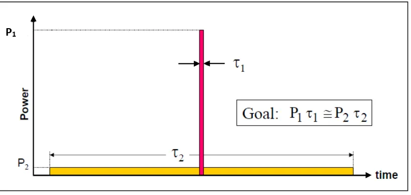
The most common radar signal or waveform, is a series of short duration, somewhat rectangular-shaped pulses modulating a sine wave carrier [3] . Short pulses are better for range resolution, but contradict with energy, long range detection, carrier frequency and SNR. Long pulses are better for signal reception, but contradict with range resolution and minimum range. At the transmitter, the signal has relatively small amplitude for ease to generate and is large in time to ensure enough energy in the signal as shown in Figure 1.1. At the receiver, the signal has very high amplitude to be detected and is small in time [4].

A very long pulse is needed for some long-range radar to achieve sufficient energy to detect small targets at long range. But long pulse has poor resolution in the range dimension.

Figure 1.1: Transmitter and receiver ultimate signals

Frequency or phase modulation can be used to increase the spectral width of a long pulse to obtain the resolution of a short pulse. This is called “pulse compression”.

3

1.2 Problem Statements

The sidelobe which is as a result of reflection affects the signal causing wastage of energy needed for wide range. It is often essential that the time (range) sidelobes of the autocorrelation function of the binary phase-coded pulses be reduced to as low level as possible, particularly in multiple-target environments that large undesired reflectors (point clutter) or in distributed clutter are available, else the time sidelobes of one large target may appear as a smaller target at another range, or the integrated sidelobes from extended targets or clutter may mask all the interesting structure in a scene [3] . Several pulse compression techniques has been proposed by various researchers and are used in many modern radar signal processing systems to reducing the effects of sidelobe by improving the accuracy of narrow pulse and retaining the capability of long pulse detection [5, 6].

1.3 Objectives of Project

The major objective of this project is to study the characterization of Radar signal measurable objectives are as follows:

1. To design pulse compression biphase codes of various length for Radar signal having lower peak sidelobes.

2. To develop sidelobe reduction method using wavelet neural networks to improve the performance of radar.

3. To compare the proposed method Wavelet neural Network (WNN) with the existing methods.

1.4 Scopes of Project

 Generate various lengths for the Phase-Coded Pulse signal in Barker code form using code.

 Artificial Neural Network (ANN) will be used to evaluate the sidelobe reduction.

 The MATLAB Version (R2013a) program will be used to simulate the study in this project.

5

1.5 Research Structure

I. Chapter 1 gives an overview of the project design. It covers the introduction to Radar and, problem statement, objectives, significant and the scope of work in this project.

II. Chapter 2 gives explanation on the pulse compression, its applications, its advantages and disadvantages. This chapter also discuss neural network and how it been constructed. Finally this chapter shows the previous studies that related to neural network.

III. Chapter 3 discussed the procedure of generating the signal and the procedure of constructing feedforward neural network (FFNN) and wavelet neural network (WNN). This chapter also explains the way of implementation of wavelet neural network to separate sidelobe.

IV. Chapter 4 presents the results obtained from the simulation process and compares these results with the results of previous studies. In this chapter, the analyzing of the results to evaluate the performance has been done.

CHAPTER 2

LITERATURE REVIEW

In radar signal transmission, pulse compression causes sidelobes. It is unwanted by-products of the pulse compression process. Sidelobe reduction techniques continue to be of interest, particularly in the case of relatively short binary codes which have the comparatively high level of sidelobes [8]. This chapter presents a review of works that deals with Pulse Compression, and sidelobe reduction using Artificial Neural Network (ANN) method as well as adaptive filters.

2.1 Pulse Compression

7

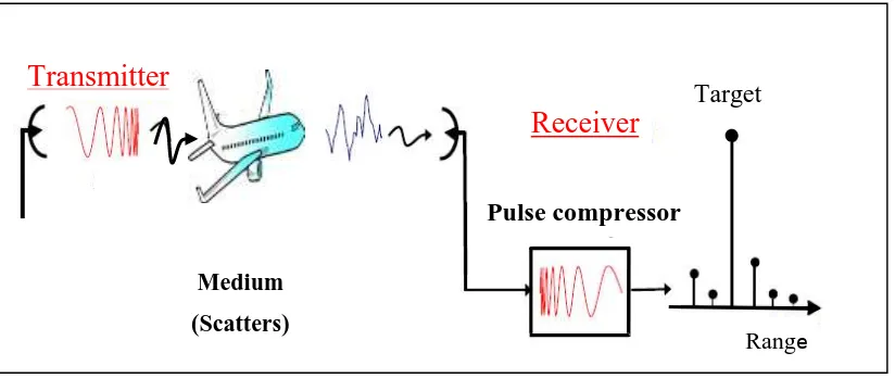
So, pulse compression permits radar to get the resolution of a short pulse and simultaneously using long waveforms so as to obtain high energy and that can be achieved by internal modulation of the long pulse [11]. The transmitted pulse is modified by using frequency modulation or phase modulation.

Figure 2.1: Concept of Pulse Compression

Then, upon receiving an echo, the received signal is compressedthrough a filter and the output signal will look like the one. It consists of a peak component and some side lobes. Figure 2.1 demonstrates the idea in simple way. The approaches by Rihaczek and Golden [12] and Baghel and Panda [8] have obtained high level of sidelobe reduction using pulse compression filter. However, this increases a computational burden and limits real time possibilities of the hardware filter applications. Pulse compression systems require advanced and expensive technology for production.

2.1.1 Advantages and Limitations of Pulse Compression

To make good range resolution and accuracy compatible with a high detection capability while maintaining the low average transmitted power, pulse compression processing giving low-range sidelobes is necessary.

Pulse compressor

Transmitter

Target

Medium

(Scatters)

(

Range

According to Melvin and Scheer [10] the principle advantages of pulse compression are as follows:

1. Increasing system resolving-capability both in range and velocity. 2. Improving signal-to-noise ratio.

3. To get a pulse–hiding transmission and thereby making the condition more difficult to the enemy to detect the "code" pulse and know whether there is a radar transmission illuminating the enemy's receiver.

4. More efficient use of the average power available at the radar transmitter and in some cases avoidance of peak power problems in the high power sections of the transmitter.

5. Extraction of information from the signals presents at the receiver input to obtain an estimation of important parameters associated with the individual signals, such as range, velocity, and possibly acceleration.

6. Increased system accuracy in measuring range and velocity. 7. Reducing clutter effects by improving the signal-to-noise ratio.

8. Increased immunity to certain types of interfering signals that do not have the same properties as the coded pulse compression waveform.

2.1.2 Pulse Compression Modulation Techniques

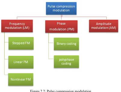
Pulse compression can be accomplished by utilizing Frequency or Phase modulation to broaden the signal bandwidth such as in Figure 2.2. Amplitude modulation is also probable but is seldom used. The transmitted pulse width (T) is chosen to achieve the single-pulse transmit energy (Et) which is required for target detection or tracking [13].

Et= Pt T (2.1)

9

Figure 2.2: Pulse compression modulation

2.1.3 Pulse Compression Effects

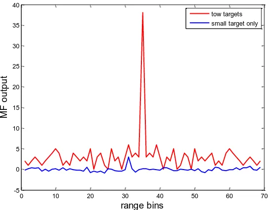
The major drawback to the pulse compression is the appearance of range sidelobes around the main signal peak which leads to smearing of the return signals in range and introduces range ambiguities [14]. The existence of a small target may not be inferred from the matched filter output when there are a small target and a large target whose power is 10 dB larger than the small one. Although the small target is noticeable when it is the only present target in the environment, in the existence of the large target the small target is masked by the range sidelobes of the large target Figure 2.3 shows Matched filter output.

Pulse compression modulation

Frequency modulation (LM)

Stepped FM

Linear FM

Nonlinear FM

Phase modulation (PM)

Binary coding

polyphase coding

Figure 2.3: Matched filter output of received radar signal

It is possible that large sidelobes can result in detecting spurious targets that are sidelobes can be mistaken as real targets. Since high sidelobes of the bigger targets can mask nearby smaller targets, suppression of range sidelobes is critical, especially in applications with multiple target systems. This effect is tried to be minimized by using carefully chosen pairs of codes or by amplitude weighting the long pulse over its duration. In general, it is not very easy to design codes with very low sidelobes. Moreover, it may not be efficient to use amplitude weighting in respect of power efficiency.

2.2 Correlation

Correlation can be defined as similar operation of the convolution. It involves sliding one function past the other and finding the area under the resulting product [15]. Unlike convolution, however, no folding is performed. The correlation 𝑟_𝑥𝑥(𝑡) of two identical functions 𝑥(𝑡) or The convolution x(t)⋆ x(−t) is called autocorrelation. For two different functions 𝑥(𝑡) and 𝑦(𝑡), the correlation 𝑟_𝑥𝑦(𝑡) or 𝑟_𝑦𝑥(𝑡) is referred to as cross-correlation.

Using the symbol ⋆⋆ to denote correlation, we define the two operations as

0 10 20 30 40 50 60 70

11

𝑟_𝑥𝑥(𝑡) = 𝑥(𝑡) ⋆⋆ x(t) = ∫ 𝑥(𝜆)𝑥( ∞

−∞

𝜆 − 𝑡) 𝑑𝜆

𝑟_𝑥𝑦(𝑡) = 𝑥(𝑡) ⋆⋆ y(t) = ∫ 𝑥(𝜆)𝑦( ∞

−∞

𝜆 − 𝑡) 𝑑𝜆

𝑟_𝑦𝑥(𝑡) = 𝑥(𝑡) ⋆⋆ x(t) = ∫ 𝑦(𝜆)𝑥( ∞

−∞

𝜆 − 𝑡) 𝑑𝜆

The variable t is often referred to as the lag. The definitions of cross- correlation are not standard, and some authors prefer to switch the definitions of 𝑟_𝑥𝑦(𝑡) and 𝑟_𝑦𝑥(𝑡).

2.2.1 Properties of Correlation

Correlations of sequences Correlation is a measure of similarity between different functions and, operation used in many applications in digital signal processing. It is a measure of the degree to which two sequences are similar [16]. Given two real-valued sequences 𝑥(𝑛) and 𝑦(𝑛) of finite energy, the cross-correlation of 𝑥(𝑛) and 𝑦(𝑛) is a sequence 𝑟_𝑥𝑦(𝑙) defined as

𝑟_𝑥,𝑦(𝑙) = ∑ 𝑥(𝑛)𝑦(𝑛 − 𝑙) ∞

𝑛=−∞

The index 𝑙is called the shift or lag parameter. The special case of (2.3).

 Correlation as Convolution

The absence of folding actually implies that the correlation of 𝑥(𝑡) and 𝑦(𝑡) is equivalent to the convolution of 𝑥(𝑡) with the folded version 𝑦(−𝑡), and we have 𝑟𝑥𝑦(𝑡) = 𝑥(𝑡) ⋆⋆ y(t) = 𝑥(𝑡) ⋆ y(−t).

(2.2)

 Area and Duration

Since folding does not affect the area or duration, the area and duration properties for convolution also apply to correlation. The starting and ending time for the cross-correlation 𝑟_𝑥𝑦(𝑡) may be found by using the starting and ending times of 𝑥(𝑡) and the folded signal 𝑦(𝑡).

 Commutation

The absence of folding means that the correlation depends on which function is shifted and, in general, 𝑥(𝑡) ⋆⋆ y(t) ≠ 𝑦(𝑡) ⋆ x(t). Since shifting one function to the right is actually equivalent to shifting the other function to the left by an equal amount, the correlation 𝑟𝑥𝑦(𝑡) is related to𝑟𝑦𝑥(𝑡) by𝑟𝑥𝑦(𝑡) = 𝑟𝑦𝑥(−𝑡). correlation is the

convolution of one signal with a folded version of the other

𝑟𝑥ℎ(𝑡) = 𝑥(𝑡) ⋆⋆ ℎ(𝑡) = 𝑥(𝑡) ⋆ ℎ(−𝑡)

𝑟ℎ𝑥(𝑡) = ℎ(𝑡) ⋆⋆ 𝑥(𝑡) = ℎ(𝑡) ⋆ 𝑥(−𝑡)

Periodic Correlation

The correlation of two periodic signals or power signals is defined in the same sense as periodic convolution:

𝑟_𝑥𝑦(𝑡) = 1

𝑇∫ 𝑥(𝜆)𝑦(𝜆 − 𝑡)𝑑𝜆 _𝑇 𝑟𝑥𝑦(𝑡) = lim𝑇0→∞

1

𝑇₀∫ 𝑥(𝜆)𝑦(𝜆 − 𝑡)𝑑𝜆_𝑇

0

The first form defines the correlation of periodic signals with identical periods T, which is also periodic with the same period T. The second form is reserved for no periodic power signals or random signals.

(2.5)

13

2.2.2 Autocorrelation

The autocorrelation operation involves identical functions. It can thus be performed in any order and represents a commutative operation. Autocorrelation may be viewed as a measure of similarity, or coherence, between a function 𝑥(𝑡) and its shifted version. Clearly, under no shift, the two functions “match” and result in a maximum for the autocorrelation. But with increasing shift, it would be natural to expect the similarity and hence the correlation between 𝑥(𝑡) and its shifted version to decrease. As the shift approaches infinity, all traces of similarity vanish, and the autocorrelation decays to zero.

 Symmetry

Since 𝑟𝑥𝑦(𝑡) = 𝑟𝑦𝑥(−𝑡) we have 𝑟𝑥𝑥(𝑡) = 𝑟𝑥𝑥(−𝑡). This means that the

autocorrelation of a real function is even. The autocorrelation of an even function 𝑥(𝑡)

also equals the convolution of 𝑥(𝑡) with itself, because the folding operation leaves an even function unchanged.

 Maximum Value

It turns out that autocorrelation function is symmetric about the origin where it attains its maximum value. It thus satisfies

𝑟_𝑥𝑥(𝑡)≤ 𝑟_𝑥𝑥(0) It follows that the autocorrelation 𝑟_𝑥𝑥(𝑡) is finite and nonnegative for all t.

 Periodic Autocorrelation

For periodic signals, we define periodic autocorrelation in much the same way as periodic convolution. If we shift a periodic signal with period 𝑇 past itself, the two line up after every period, and the periodic autocorrelation also has period 𝑇.

2.2.3 Matched Filters

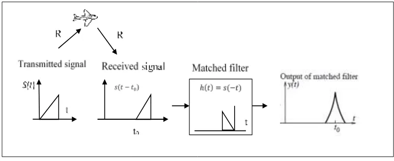
Correlation forms the basis for many methods of signal detection and delay estimation (usually in the presence of noise). An example is target ranging by radar, illustrated in Figure 2.4, where the objective is to estimate the target distance (or range) R.

Figure 2.4: Illustrating the concept of matched filtering

A transmitter sends out an interrogating signal𝑠(𝑡), and the reflected and delayed signal (the echo) s(t − t0) is processed by a correlation receiver, or matched filter, whose impulse response is matched to the signal to obtain the target range. In fact, its impulse response is chosen as h(t) = s(−t), a folded version of the transmitted signal, in order to maximize the signal-to-noise ratio. The response y(t) of the matched filter is the convolution of the received echo and the folded signal h(t) = s(−t) or the correlation of s(t−t0) (the echo) and s(t) (the signal). This response attains a maximum

at t = t0, which represents the time taken to cover the round-trip distance 2R. The target

range R is then given by

𝑅 = 𝑐𝑡0 2

where c is the velocity of signal propagation.

15

original signal (as it usually is), their cross-correlation is very small (ideally zero), and the cross-correlation of the original signal with the noisy echo yields a peak (at t = t0) that stands out and is much easier to detect. Ideally, of course, we would like to transmit narrow pulses (approximating impulses) whose autocorrelation attains a sharp peak [15].

2.3 Neural Network

The neural network is defined by [17] as a massively parallel distributed processor made up of simple processing units, which has a natural propensity for storing experiential knowledge and making it available for use. The system emulates the brain in two ways as described below.

i. Knowledge is acquired by the network from its environment through a learning process.

ii. Interneuron connection strengths, known as synaptic weights, are used to store the acquired knowledge.

2.3.1 Biological Neuron Model

The human brain consists of more than billions of neural cells that process information. Each cell works like a simple processor. The massive interaction between all cells and their parallel processing only makes the brain's abilities possible.

The Biological Neuron as shown in Figure 2.5 consists of the following:

Dendrites: are branching fibers that extend from the cell body or soma. Soma or cell body of a neuron contains the nucleus and other structures, support chemical processing and production of neurotransmitters.

of all neurons that conduct impulses to a given neuron will determine whether or not an action potential will be initiated at the axon hillock and propagated along the axon.

Figure 2.5: Structure of Biological Neuron [18]

Myelin Sheath: consists of fat-containing cells that insulate the axon from the electrical activity. This insulation acts to increase the rate of transmission of signals. A gap exists between each myelin sheath cell along the axon. Since fat inhibits the propagation of electricity, the signals jump from one gap to the next.

Nodes of Ranvier: are the gaps (about 1μm) between myelin sheath cells long axons are since fat serves as a good insulator, the myelin sheaths speed the rate of transmission of an electrical impulse along the axon.

17

2.3.2 Artificial Neural Network

An Artificial Neural Network (ANN) is an information-processing paradigm that is inspired, by the way, the biological nervous system such as brain process information [19, 20]. The first artificial neuron was developed in 1943 by the neurophysiologist Warren McCulloch and the logician Walter Pits. But the technology available at that time did not allow them to proceed further. In past few decades, the ANN has emerged as a powerful learning tool to perform complex tasks in the highly nonlinear dynamic environment. The ANN is capable of performing nonlinear mapping between the input and output space due to its large parallel interconnection between different layers and the nonlinear processing characteristic. Therefore, the ANN is used extensively in the field of communication, some control systems, instrumentation and forecasting [21, 22]. ANN technique is also used for classification, modeling and optimization problems [23].

An artificial neuron basically consists of a computing element that performs the weighted sum of the input signal and the connecting weight. The sum is added with the bias or threshold and the resultant signal is then passed through an activation function of the sigmoid or hyperbolic tangent type. Each neuron is associated with three parameters whose learning can be adjusted. These are the connecting weights, the bias and the slope of the nonlinear function. For the structural point of view, a neural network (NN) may be a single layer or it may be multilayer. In Multi-layer Perceptron MLP, there is a number of layers and each layer contains one or many artificial neurons. Each neuron of the one layer is connected to each and every neuron of the next layer. A trained neural network can be thought of as an “expert” in the category of information it has been given to analyze. The advantages of ANN are:

a) Adaptive learning: It is the ability of the network to learn how to do tasks based on the data given for training or initial experience.

c) Real-time operation: The ANN computations may be carried out in parallel, and special hardware devices are being designed and manufactured which take advantage of this capability.

d) Fault tolerance via redundant information coding: Partial destruction of a network leads to the corresponding degradation in performance. However, some network capabilities may be retained even with major network damage.

The structure of ANN is described as follow:

I. Single Neuron Structure

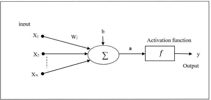
A neuron is an information processing unit for the operation of a neural network. The operation in a single neuron involves the computation of the weighted sum of inputs and threshold [23]. The resultant signal is then passed through activation function. The activation functions can be defined as a limiting the amplitude of the output of the neuron and it is also called a squashing function in that it squashes (limits) the permissible amplitude range of the output signal to the some finite value. The neuronal model also includes an externally applied bias, expressed by bi, the bias bi has the effect of increasing or lowering the net input of the activation function, depending on whether it is positive or negative, respectively. The basic structure of a single neuron is shown in Figure 2.6.

Figure 2.6: Single neuron structure

𝑓

∑

input

Output X1

XN

b

a

Activation function

19

In mathematical terms, we may describe a neuron 𝐾 by writing the following pair of equations:

𝑎𝑘 = ∑ 𝑊𝑘𝑗𝑋𝑗 𝑁

𝑗=1

The output associated with the neuron is computed as

Y=𝑓[∑𝑁 _𝑖=1 𝑎𝑖 + b] (2.11)

Where xi, i = 1, 2...N, are inputs to the neuron; wi is the synaptic weights of the ith

input; b is the bias; 𝑓 is the activation function for each neuron; and y is the output signal of the neuron. The use of bias (b) has the effect of applying an affine transformation to the output (a). The most common types of activation function are discussed below [23].

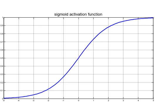
 Log-sigmoid function

This transfer function takes the input and squashes the output into the range of 0 to 1, according to expression given below:

𝑓(𝑥) =

1+𝑒−𝑥 (2.12)

Figure 2.7: The sigmoid activation function

-5 -4 -3 -2 -1 0 1 2 3 4 5

0 0.1 0.2 0.3 0.4 0.5 0.6 0.7 0.8 0.9

1 sigmoid activation function

 Hyperbolic tangent Sigmoid:

This function is expressed in equation 2.13

𝑓(𝑥) = tanh(x) =

x_−e−x

ex_+e−x (2.13)

Figure 2.8: Tansig activation function

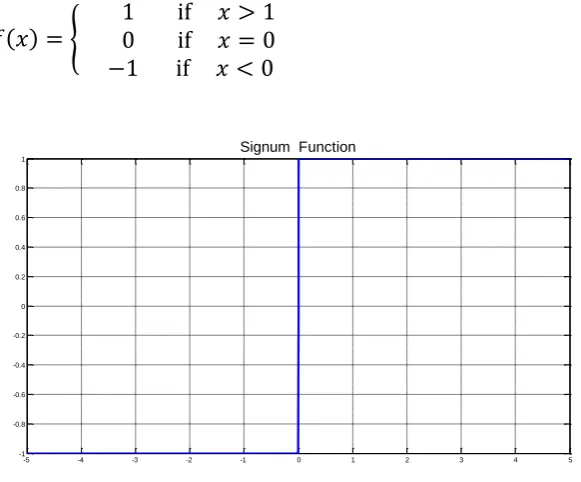
 Signum Function:

The expression for this activation function is given by

𝑓(𝑥) = {

1 if 𝑥 > 1 0 if 𝑥 = 0 −1 if 𝑥 < 0

(2.14)

Figure 2.9: Signum activation Function

-5 -4 -3 -2 -1 0 1 2 3 4 5

-1 -0.8 -0.6 -0.4 -0.2 0 0.2 0.4 0.6 0.8 1

tansig activation function

-5 -4 -3 -2 -1 0 1 2 3 4 5

-1 -0.8 -0.6 -0.4 -0.2 0 0.2 0.4 0.6 0.8 1

21

 Threshold function

This function is given by the expression

𝑓(𝑥) = {

1 if 𝑥 ≥ 1

0 if 𝑥 < 0

(2.15)

 Piecewise linear function This function is represented as

𝑓(𝑥) = {

1 if 𝑥 > 0.5 𝑥 if − 0.5 ≤ 𝑥 ≤ 0.5

−1 if 𝑥 < 0.5

(2.16)

II. ANN learning

Learning rules mean the procedure by which modifying the weights and biases of ANN, this procedure may also be referred to as training algorithm, the purpose of learning rule is to train the network to perform some special tasks. There are many types of NNs learning rules; they fall into three basic categories: supervised learning, unsupervised learning, and reinforcement learning [24].

In supervised learning, the learning rules are provided with a set of examples (training set) of proper network behavior. Supervised learning rewards accurate classifications or associations and punishes those which yield inaccurate responses. The teacher estimates the negative error gradient direction and reduces the error accordingly [24].

(a) The Selecting appropriate number of hidden layers in the network. (b) Selecting the number of neurons to be used in each hidden layer. (c) Finding a globally optimal solution, that avoids local minima. (d) Converging to an optimal solution in a reasonable period of time. (e) Validating the neural network to test for over-fitting.

Depending on the architecture in which the individual neurons are connected and the choice of the error minimization procedure, there can be several possible ANN configurations.

2.4 Wavelet Analysis

Wavelet analysis is a mathematical tool used in various areas of research. Recently, wavelets have been used especially to analyze time series, data, and images. Time series are represented by local information such as frequency, duration, intensity, and time position, and by global information such as the mean states over different time periods [27]. Both global and local information is needed for the correct analysis of a signal. The Wavelet Transform (WT) is a generalization of the Fourier Transform (FT) and the Windowed Fourier Transform (WFT).

A wavelet 𝜓 is a waveform of effectively limited duration that has an average value of zero. The Wavelet Analysis (WA) procedure adopts a particular wavelet function called a mother wavelet. A wavelet family is a set of orthogonal basis functions generated by dilation and translation of a compactly supported scaling function 𝜑 (or father wavelet), and a wavelet function 𝜓 (or mother wavelet). The father wavelets 𝜑 and mother wavelets 𝜓 satisfy

∫ 𝜑(𝑡) 𝑑𝑡 = 1

23

The wavelet family consists of wavelet children which are dilated and translated forms of a mother wavelet:

𝜓_𝑎,𝑏(𝑡) = 1 √𝑎𝑗

𝜓 (𝑡 − 𝑏 𝑎 )

where a is the scale or dilation parameter and b is the shift or translation parameter. The value of the scale parameter determines the level of stretch or compression of the wavelet. The term 1 √𝑎⁄ normalizes‖𝜓𝑎,𝑏(𝑡)‖ = 1.

In general, wavelets can be separated in orthogonal and nonorthogonal wavelets. The term wavelet function is used generically to refer to either orthogonal or nonorthogonal wavelets. An orthogonal set of wavelets is called a wavelet basis, and a set of nonorthogonal wavelets is termed a wavelet frame. The use of an orthogonal basis implies the use of the Discrete Wavelet Transform (DWT), whereas frames can be used with either the discrete or the continuous transform.

Over the years a substantial number of wavelet functions have been proposed in the literature. The Gaussian, the Morlet, and the Mexican hat wavelets are crude wavelets that can be used only in continuous decomposition. The wavelets in the Meyer wavelet family are infinitely regular wavelets that can be used in both Continues Wavelet Transform (CWT) and DWT. The equations that represent the Gaussian, Morlet, Shannon, Meyer and Mexican hat wavelet families are presented In the next sections [27].

2.5 Wavelet Neural Network

Wavelet networks are a new class of networks that combine the classic sigmoid neural networks and wavelet analysis. Wavelet networks were proposed by Zhang and Benveniste [28] as an alternative to feedforward neural networks which would alleviate the weaknesses associated with wavelet analysis and neural networks while preserving the advantages of each method.

classification and compression; signal denoising; static, dynamic, and nonlinear modeling; to nonlinear static function approximation [27].

Wavelet networks are hidden layer networks that use a wavelet for activation instead of the classic sigmoidal family. It is important to mention here that multidimensional wavelets preserve the “universal approximation” property that characterizes neural networks. The nodes (or wavelons) of wavelet networks are wavelet coefficients of the function expansion that have a significant value. Bernard, Mallat [29], various reasons were presented for why wavelets should be used instead of other transfer functions as illustrated in points below:

1. wavelets have high compression abilities.

2. computing the value at a single point or updating a function estimate from a new local measure involves only a small subset of coefficients.

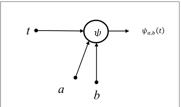
2.5.1 Single Wavelet Neuron Structure

The structure of the single wavelet neuron is the same as the neural network structure. neural network is one with a single input and a single output. The hidden layer of neurons consist of hidden layer (wavelons), whose input parameters (possibly fixed) include the wavelet dilation and translation coefficients. These wavelons produce a non-zero output when the input lies within a small area of the input domain. The output of a wavelet neural network is a linear weighted combination of the wavelet activation functions. Figure 2.10 shows the single Wavelet Neuron Structure.

Figure 2.10: Single Wavelet Neuron Structure

𝜓

t

80

REFERENCES

1. Raju, G., Radar engineering. 2008, New Delhi: IK International Pvt Ltd. 2. Merrill, I.S., Introduction to radar systems. Mc Grow-Hill, 2001.

3. Nathanson, F.E., J. Reilly, and M.N. Cohen, Radar design principles-Signal processing and the Environment. NASA STI/Recon Technical Report A, 1999. 91: p. 46747.

4. Darwich, T., High resolution detection systems using low sidelobe pulse compression techniques. 2007: University of Louisiana at Lafayette.

5. Duh, F.-B., C.-F. Juang, and C.-T. Lin, A neural fuzzy network approach to radar pulse compression. Geoscience and Remote Sensing Letters, IEEE, 2004. 1(1): p. 15-20.

6. Chi, Y., et al. Range sidelobe suppression in a desired Doppler interval. in Proc. IEEE Waveform Diversity and Design Conference. 2009.

7. Skolnik, M.I., Introduction to radar. Radar Handbook, 1962. 2.

8. Baghel, V. and G. Panda, Development of an efficient hybrid model for range sidelobe suppression in pulse compression radar. Aerospace Science and Technology, 2013. 27(1): p. 156-162.

9. Cao, S., Y.F. Zheng, and R.L. Ewing, Wavelet-Based Waveform for Effective Sidelobe Suppression in Radar Signal. Aerospace and Electronic Systems, IEEE Transactions on, 2014. 50(1): p. 265-284.

10. Melvin, W.L. and J.A. Scheer, Principles of modern radar. 2013. II: Advanced Techniques.

11. Rao, P., et al. A novel VLSI architecture for generation of Six Phase pulse compression sequences. in Devices, Circuits and Systems (ICDCS), 2012 International Conference on. 2012. IEEE.

13. Darwich, T. and C. Adviser-Cavanaugh, High resolution detection systems using low sidelobe pulse compression techniques. 2007: University of Louisiana at Lafayette.

14. Haliloglu, O., successive target cancelation for radar waveform sidelobe reduction, 2006, middle east technical university.

15. Ambardar, A., Digital Signal Processing-A Modern Introduction. 2006: Thomson-Engineering.

16. Ingle, V. and J. Proakis, Digital signal processing using MATLAB. 2011: Cengage Learning.

17. Haykin, S. and N. Network, A comprehensive foundation. Neural Networks, 2004. 2(2004).

18. Graupe, D., Principles of artificial neural networks. Vol. 6. 2007: World Scientific.

19. Freeman, J.A. and D.M. Skapura, Neural networks: algorithms, applications, and programming techniques, 1991. Reading, Massachussets: Addison-Wesley. 20. Haykin, S.S., et al., Neural networks and learning machines. Vol. 3. 2009:

Pearson Education Upper Saddle River.

21. Vongkunghae, A. and A. Chumthong, The performance comparisons of backpropagation algorithm’s family on a set of logical functions. ECTI Transactions on Electrical Eng Electronics and Communications (ECTEEC), 2007. 5(2): p. 114-118.

22. Rabunal, J.R. and J. Dorado, Artificial neural networks in real-life applications. 2006: IGI Global.

23. Beale, M.H., M.T. Hagan, and H.B. Demuth, Neural Network Toolbox 7. User’s Guide, MathWorks, 2010.

24. Hamed, H.N.A., S.M. Shamsuddin, and N. Salim, Particle Swarm Optimization For Neural Network Learning Enhancement. Jurnal Teknologi, 2012. 49(1): p. 13–26.

25. Liu, Y., J.A. Starzyk, and Z. Zhu, Optimized approximation algorithm in neural networks without overfitting. Neural Networks, IEEE Transactions on, 2008. 19(6): p. 983-995.

82

27. Alexandridis, A.K. and A.D. Zapranis, Wavelet Neural Networks: With Applications in Financial Engineering, Chaos, and Classification. 2014: John Wiley & Sons.

28. Zhang, Q. and A. Benveniste, Wavelet networks. Neural Networks, IEEE Transactions on, 1992. 3(6): p. 889-898.

29. Bernard, C.P., S. Mallat, and J.-J.E. Slotine. Wavelet interpolation networks. in ESANN. 1998. Citeseer.

30. Wang, G., L. Guo, and H. Duan, Wavelet neural network using multiple wavelet functions in target threat assessment. The Scientific World Journal,2013: p. 7. 31. Cristea, P., R. Tuduce, and A. Cristea. Time series prediction with wavelet

neural networks. in Neural Network Applications in Electrical Engineering, 2000. NEUREL 2000. Proceedings of the 5th Seminar on. 2000. IEEE.

32. Lin, C.-H., Y.-C. Du, and T. Chen, Adaptive wavelet network for multiple cardiac arrhythmias recognition. Expert Systems with Applications, 2008. 34(4): p. 2601-2611.

33. He, K., K.K. Lai, and J. Yen, Ensemble forecasting of Value at Risk via Multi Resolution Analysis based methodology in metals markets. Expert Systems with Applications, 2012. 39(4): p. 4258-4267.

34. Xu, J. and D.W. Ho, A constructive algorithm for wavelet neural networks, in Advances in Natural Computation. 2005, Springer. p. 730-739.

35. Chen, Y., B. Yang, and J. Dong, Time-series prediction using a local linear wavelet neural network. Neurocomputing, 2006. 69(4): p. 449-465.

36. Zhang, Z., Iterative algorithm of wavelet network learning from nonuniform data. Neurocomputing, 2009. 72(13): p. 2979-2999.

37. Yao, X., Evolving artificial neural networks. Proceedings of the IEEE, 1999. 87(9): p. 1423-1447.

38. Zhang, Q. Regressor selection and wavelet network construction. in Decision and Control, 1993., Proceedings of the 32nd IEEE Conference on. 1993. IEEE. 39. Zhang, Q., Using wavelet network in nonparametric estimation. 1994.

40. ZHANG, Q., USING WAVELET NETWORK IN NONPARAMETRIC ESTIMATION. 1997.

42. Jiao, L., J. Pan, and Y. Fang, Multiwavelet neural network and its approximation properties. Neural Networks, IEEE Transactions on, 2001. 12(5): p. 1060-1066. 43. Oussar, Y. and G. Dreyfus, Initialization by selection for wavelet network

training. Neurocomputing, 2000. 34(1): p. 131-143.

44. Postalcioglu, S. and Y. Becerikli, Wavelet networks for nonlinear system modeling. Neural Computing and Applications, 2007. 16(4-5): p. 433-441. 45. Oussar, Y., et al., Training wavelet networks for nonlinear dynamic input–

output modeling. Neurocomputing, 1998. 20(1): p. 173-188.

46. Zapranis, A. and A.-P. Refenes, Principles of Neural Model Identification, Selection and Adequacy: With Applications to Financial Econometrics. 1999: Springer Science & Business Media.

47. Zhao, J., W. Chen, and J. Luo, Feedforward wavelet neural network and multi-variable functional approximation, in Computational and Information Science. 2005, Springer. p. 32-37.

48. Wiener, N., Extrapolation, interpolation, and smoothing of stationary time series. Vol. 2. 1949: MIT press Cambridge, MA.

49. Akbaripour, A. and M.H. Bastani, Range sidelobe reduction filter design for binary coded pulse compression system. Aerospace and Electronic Systems, IEEE Transactions on, 2012. 48(1): p. 348-359.

50. Vaseghi, S.V., Advanced digital signal processing and noise reduction. 2008: John Wiley & Sons.

51. Gen-miao, Y., W. Shun-jun, and L. Yong-jian. Doppler properties of polyphase pulse compression codes under different side-lobe reduction techniques. in Radar, 2001 CIE International Conference on, Proceedings. 2001. IEEE. 52. Fu, X., L. Tian, and M. Gao. Sidelobe suppression of LPI phase-coded radar

signal. in Radar Systems, 2007 IET International Conference on. 2007. IET. 53. Khairnar, D., S. Merchant, and U. Desai, Radial basis function neural network

for pulse radar detection. IET Radar, Sonar & Navigation, 2007. 1(1): p. 8-17. 54. Padaki, A.V. and K. George. Improving performance in neural network based

pulse compression for binary and polyphase codes. in Computer Modelling and Simulation (UKSim), 2010 12th International Conference on. 2010. IEEE. 55. Sailaja, A., New Approaches to Pulse Compression Techniques of Phase-Coded

84

56. Sahoo, A.K., G. Panda, and B. Majhi. A technique for pulse radar detection using RRBF neural network. in The 2012 International Conference of Computational Intelligence and Intelligent Systems London, UK, 4-6 July 2012. 2012.

57. Fu, J.S. and X. Wu. Sidelobe suppression using adaptive filtering techniques. in Radar, 2001 CIE international conference on, proceedings. 2001. IEEE. 58. Sahoo, A.K., Development of Radar Pulse Compression Techniques Using

Computational Intelligence Tools, 2012, PhD thesis with National Institute of Technology Rourkela

59. Hafez, A. and M.A. El-latif. New radar pulse compression codes by particle swarm algorithm. in Aerospace Conference, 2012 IEEE. 2012. IEEE.

60. Vizitiu, I.-C., Sidelobe reduction in the pulse-compression radar using synthesis of NLFM laws. International Journal of Antennas and Propagation, 2013. 61. Mahafza, B.R., Radar Systems Analysis and Design Using MATLAB Third

Edition. 2013: CRC Press.

62. Levanon, N. and E. Mozeson, Radar signals. 2004: John Wiley & Sons. 63. Meikle, H., Modern radar systems. 2008: Artech House.