Theory and Applications of the Multiwavelets
for compression of Boundary Integral
Operators.
Steven Paul Nixon B.Sc.
Institute for Materials Research
School of Computing, Science & Engineering,
University of Salford, Salford, UK.
Contents
1 Introduction 1
2 Boundary Integral Methods 6
2.1 Sobolev Spaces . . . 7
2.2 Pseudodifferential Operators . . . 9
2.2.1 Solvability of Pseudodifferential Operator Equations . . . 12
2.3 Boundary Integral Equations . . . 14
2.3.1 Free Space Green’s Function . . . 14
2.3.2 Boundary Integral Operators . . . 15
2.3.3 Direct Formulation of the Boundary Integral Equation . . . 17
2.4 Projection Methods . . . 18
2.4.2 Galerkin Method . . . 21
3 Wavelet Analysis 24 3.1 Multiresolution . . . 25
3.1.1 Multiscale Basis . . . 27
3.1.2 Vanishing Moments . . . 29
3.1.3 Multiscale Transformations . . . 32
3.1.4 Wavelets on[0,1] . . . 43
3.2 Multiwavelets on[0,1] . . . 44
3.2.1 Multiwavelet Construction . . . 47
3.2.2 Multiwavelet Approximation . . . 50
3.2.3 Multiwavelet Transformations . . . 51
4 Multiwavelet Galerkin Methods 60 4.1 The Standard Galerkin Method . . . 61
4.1.1 Matrix Element Bounds . . . 62
4.1.2 Compression Strategy . . . 65
4.2.1 Matrix Element Bounds . . . 79
4.2.2 Compression Strategy . . . 81
5 The Radiosity Problem 87 5.1 Radiometric Quantities . . . 88
5.2 The Radiosity Equation . . . 90
5.2.1 Numerical Results . . . 93
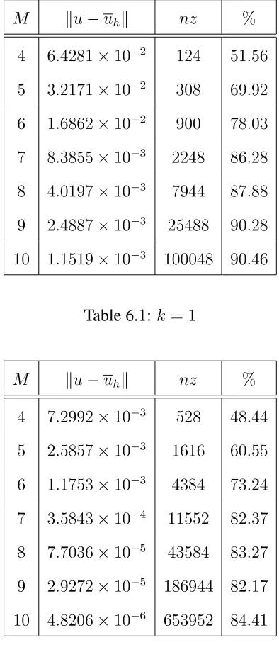
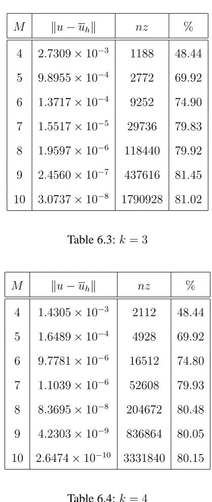
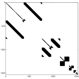
6 Numerical Solution of Laplace’s Equation 107 6.1 The Neumann Problem . . . 108
6.1.1 Numerical Results . . . 109
6.2 The Dirichlet Problem . . . 126
6.2.1 Preconditioning . . . 127
6.2.2 Wavelet Preconditioning . . . 128
6.2.3 Multiwavelet Preconditioning . . . 129
6.2.4 Numerical Results . . . 130
7 Conclusion and Further work 137
Acknowledgements
I would like to thank my supervisor Professor Sia Amini for his help, support and
encour-agement. I am also grateful to EPRSC for their financial support. My parents, as always
have been very supportive and understanding. Finally, I would like to thank everyone in
Abstract
In general the numerical solution of boundary integral equations leads to full coefficient
matrices. The discrete system can be solved in O(N2)operations by iterative solvers of
the Conjugate Gradient type. Therefore, we are interested in fast methods such as fast
multipole and wavelets, that reduce the computational cost toO(NlnpN).
In this thesis we are concerned with wavelet methods. They have proved to be very
efficient and effective basis functions due to the fact that the coefficients of a wavelet
ex-pansion decay rapidly for a large class of functions. Due to the multiresolution property
of wavelets they provide accurate local descriptions of functions efficiently. For example
in the presence of corners and edges, the functions can still be approximated with a
lin-ear combination of just a few basis functions. Wavelets are attractive for the numerical
solution of integral equations because their vanishing moments property leads to operator
compression. However, to obtain wavelets with compact support and high order of
van-ishing moments, the length of the support increases as the order of the vanvan-ishing moments
increases. This causes difficulties with the practical use of wavelets particularly at edges
and corners. However, with multiwavelets, an increase in the order of vanishing moments
is obtained not by increasing the support but by increasing the number of mother wavelets.
In chapter 2 we review the methods and techniques required for these reformulations,
we also discuss how these boundary integral equations may be discretised by a boundary
element method. In chapter 3, we discuss wavelet and multiwavelet bases. In chapter
4, we consider two boundary element methods, namely, the standard and non-standard
Galerkin methods with multiwavelet basis functions. For both methods compression
strategies are developed which only require the computation of the significant matrix
ele-ments. We show that they are O(NlogpN)such significant elements. In chapters 5 and
Chapter 1
Introduction
Over the last three-to-four decades it has become popular to reformulate linear second
order partial differential equations as integral equations over the boundary of the region
of interest. These boundary integral equations are then solved by finite element type
dis-cretisations; referred to as boundary element methods (BEM). Our research is concerned
with methods for solving boundary integral equations with almost optimal efficiency.
There are several advantages to using BEM in place of finite element methods (FEM)
applied to the original partial differential equation, see [1]:
• Exterior problems are treated more naturally, since BEM requires meshing over
only a finite domain, whereas, FEM requires meshing over an infinite domain.
Boundary conditions at infinity can be neatly incorporated into the boundary
• Reformulating the problem on the boundary alone reduces the dimension of the
problem by one, resulting in smaller matrices for the same mesh sizeh.
• BEM allows us to compute the solution only in a subdomain of special interest.
When using FEM, the solution must be computed everywhere.
• The matrices formed by BEM are generally better conditioned than those formed
by FEM.
There are also disadvantages to BEM:
• FEM can be applied to linear, nonlinear and time-dependent partial differential
equations. Boundary element counterparts for more “complicated” partial
differ-ential equations have not yet fully developed, although research is underway, eg [2].
• The elements of matrices formed by FEM are easy to compute. By contrast, each
element of a BEM matrix involves integration. For diagonal elements, these
inte-grals may be singular.
• The matrices formed by FEM are sparse and can be solved quickly by fast solvers.
However, boundary element matrices are full. Traditionally, they are solved by a
direct method such as Gaussian elimination. However, we are interested in fast
methods which reduce the computing time for large scale problems.
Briefly, boundary element methods partition the boundary intoN elements. This results in
the system in O(N3) arithmetic operations. In general, the use of an iterative solver,
possibly with preconditioning, results in O(N2) operations. However, these methods
cannot improve upon anO(N2)complexity estimate, since simply forming the coefficient
matrix requiresO(N2)arithmetic operations.
The fast methods with which we are concerned aim to solve the boundary integral
equa-tion to within the discretisaequa-tion error in O(NlogpN)
for some small integer value p;
typicallyp = 0,1,2. This is the so-called almost optimal complexity one can achieve in
findingN-unknowns.
A typical (Galerkin) boundary element matrix entry has the form
Aij =
Z
Γ
Z
Γ
K(p,q)ψi(p)ψj(q)dΓqdΓp. (1.0.1)
Clearly, in a fast method we can not evaluate the whole coefficient matrixA. Currently,
there are two distinct classed of fast methods for solving boundary integral equations.
One is the so-called fast multipole algorithm, closely related to panel clustering [3]; see
Profit, Amini & Profit [4, 5] for application to the Helmholtz equation. The basic idea
here is that the kernelK(p,q)of the integral operator is approximated by a degenerate or
“separable” kernel
K(p,q)≈
L
X
l,m=−1
fl(p)blmgm(q) =f(p)TBg(q).
Substituting this into (1.0.1) we can see that
whereU is anN ×Lmatrix,BanL×Lmatrix, andV anL×N matrix with entries,
Uil =
Z
Γ
fl(p)ψi(p)dΓp
Blm=blm
Vmj =
Z
Γ
gm(q)ψj(q)dΓq.
In place ofAthe elements of the sparse matrix decompositionU BV are computed. This
requires 2N L+L2 elements, as opposed to N2 for A. If L = O(logN) we see that
this requires onlyO(NlogN)elements are stored and a similar number of operations for
formingA˜x.
The second type of fast method, with which we are concerned with in this thesis, is the
so-called wavelet algorithm, [6, 7, 8, 9]. Here, the basis functions ψi are the so-called
wavelet basis. These are refinable bases obtained from translations and scalings of a
single functionψ, the so-called mother wavelet. That is,
ψi = 2
m
2 ψ(2m· −l) for m∈Z, l ∈ ∇m.
They have the additional property of being orthogonal to low order polynomials; known
as the property of vanishing moments.
We can show that using a wavelet basis, for a large class of kernels the elements of the
Galerkin matrixAsatisfy,
|Aij| ≤c
2−(m+m′)(k+1 2)−2k (2k+ 1) dist(Γj,Γi)1+2k+α
.
We can prove that onlyO(NlogpN)of these elements are sufficiently large enough to
in the desired efficiency.
In chapter 2 we review the methods and techniques required when partial differential
equations are reformulated as boundary integral equations. We also discuss how these
boundary integral equations may be discretised by a boundary element method. In chapter
3, we present the multiresolution framework for wavelets, along with our choice of basis
functions for this thesis, namely, the multiwavelets of [10].
In chapter 4, we consider two boundary element methods, namely, the standard and
non-standard Galerkin methods with multiwavelet basis functions. For both methods applied
to operators of the standard analytical class, we find bounds for the size of the
coeffi-cient matrix elements. Using these bounds compression strategies are developed which
only require the computation of the significant matrix elements. We show that there are
O(NlogpN)such significant elements, for some small integer valuep.
In chapters 5 and 6 we apply the standard and non-standard Galerkin methods to
sev-eral test problems. In chapter 5 we are concerned with the radiosity problem of image
synthesis, whereas, in chapter 6 we are concerned with the boundary integral equation
re-formulation of Laplace’s equation. However, when we consider Laplace’s equation with
Dirichlet boundary conditions the resulting coefficient matrix is ill-conditioned.
There-fore, in order to use an iterative solver efficiently we must precondition the coefficient
matrix. For a wavelet basis a diagonal scaling matrix is shown to be sufficient, see [11].
Here, we extend the preconditioner for use with multiwavelet basis functions. Finally we
Chapter 2
Boundary Integral Methods
In this chapter we introduce the methods and techniques required for solving boundary
integral equations. In general boundary integral equations are derived as reformulations
of partial differential equations over a domainΩ. We arrive at equations of the form
(Au) (p) =
B∂n∂u
(p), p∈Γ =∂Ω, (2.0.1)
whereAandBare pseudodifferential operators.
To discuss the existence and uniqueness of solutions to (2.0.1) and study the convergence
analysis of boundary element methods, we need to introduce appropriate function spaces.
Sobolev spaces are introduced in section 2.1. The operators A and B are
pseudodiffer-ential operators over Sobolev spaces. This allows us to study differpseudodiffer-ential, integral and
hypersingular operators within the same framework. Pseudodifferential operators are
in-troduced in section 2.2. In section 2.3 we reformulate Laplace’s equation as a boundary
integral equation of the form (2.0.1), such equations are discretised using the projection
2.1
Sobolev Spaces
Sobolev spaces provide a natural setting in which to describe the smoothness of solutions
in partial differential theory. In this section, we briefly introduce these spaces and their
basic properties. For a more comprehensive study see [12].
Let Ω be a simply connected domain in Rn. Initially the Sobolev spaces Ws
p(Ω) are
defined for non-negative integers s. For a multi-index of non-negative integers l =
(l1, . . . , ln), we define the partial derivative Dlby
Dlx =Dl1
1Dl22. . .Dlnn =
∂l1
∂xl1
1
. . .
∂ln ∂xln
n
= ∂
|l|
∂xl1
1 . . . ∂xlnn
, (2.1.1)
where|l|=l1+. . .+ln.
Definition 2.1.1. The spaceWps(Ω)is the space defined by
Ws
p(Ω) :=
u∈Lp(Ω)|Dlu∈Lp(Ω)for |l| ≤s , (2.1.2)
and is equipped with the norm
kukWs
p =
X
|l|≤s
Z
Ω
Dlu(x)pdx
1
p
, (2.1.3)
see [13].
Sobolev spaces withp6= 2are rarely used. Therefore, we concentrate on the casep = 2
and denote W2s(Ω) by Hs(Ω). We note, that for s = 0, H0(Ω) = L
2(Ω). In order
functionu,
ˆ
u(ξ) =
Z
Ω
e−2πix.ξu(x)dx. (2.1.4)
Then, it can be shown, see [1], that for non-negative integerss,
c1kuk2Hs ≤
Z
Ω
1 +|ξ|2s|uˆ(ξ)|2dξ ≤c2kuk2Hs. (2.1.5)
Therefore,
Z
Ω
1 +|ξ|2s|uˆ(ξ)|2dξ
1 2
(2.1.6)
defines an equivalent norm inHs(Ω). Furthermore, (2.1.6) has meaning for all real values
ofs. This allows us to defineHs(Ω)for any reals, possibly negative, by
Hs(Ω) :={u∈L2(Ω)|uis a generalized function such that (2.1.6) is finite}. (2.1.7)
In fact, for0 ≤ s < ∞ the space H−s(Ω) is the dual ofHs(Ω), i.e. space of bounded
linear functionals onHs(Ω).
LetΓ be the boundary of a simply connected domainΩ ⊂ Rn. Then, we can similarly
define Sobolev spacesHs(Γ), see [1]. For the casen = 2, ifΓhas a smooth
parameteri-sation
γ : [0,1)→Γ,
then, we may defineHs(Γ)by
Hs(Γ) :={u|(u◦γ)∈Hs[0,1)}, (2.1.8)
where(u◦g)(x) =u(γ(x)). This definition is invariant under changes of the
Supposes, t∈Rwiths > t. Then, Hs ⊂Htand foru ∈Hswe havekuk
Ht ≤ kukHs. In fact the imbedding (identity) operatorI :Hs
→Htis compact, see [1, Theorem 2.1.5].
We now mention an important trace theorem, [1, Theorem 2.2.2].
Theorem 2.1.1. Let Ωbe a bounded open domain with smooth boundary Γ. If s > 12,
then the trace operator
u→ u|Γ (2.1.9)
is a continuous mapping fromHs(Ω)toHs−1 2(Γ).
2.2
Pseudodifferential Operators
Pseudodifferential operators are a natural extension of linear integral and partial
differ-ential operators. The theory of pseudodifferdiffer-ential operator has developed alongside the
study of singular integral operators, which occur in many areas of mathematical physics.
A pseudodifferential operator is a linear operator A : Hs(Ω) → Hs−α(Ω) where α is called the order of the operator. We can write the pseudodifferential operator A as the
integral operator
(Au) (p) =
Z
Ω
a(p,q)u(q)dΩq, (2.2.1)
where a(·,·)is a kernel function or a distribution. If a is a weakly singular kernel this
is a classical compact integral operator. However, this definition also covers the cases of
differential and integro-differential operators. We follow the approach of [1] to introduce
the pseudodifferential operator concept.
A general partial differential operator of orderαis a polynomial expression of the form
P(x,D) = X
|l|≤α
wherel = (l1, . . . , ln)is a multi-integer and the symbol of the operatorP is defined by
σ(P) =p(x, ξ) = X
|l|≤α
al(x) (iξ)l. (2.2.3)
Therefore, we wish to show that P u can be written in the integral form (2.2.1). We
consider the inverse Fourier transform
u(x) =
Z
Ω
e2πix.ξuˆ(ξ)dξ. (2.2.4)
It follows that the partial derivatives satisfy
Dlxu(x) =
Z
Ω
e2πix.ξ(2πiξ)luˆ(ξ)dξ, (2.2.5)
and hence,
P(x,D)u(x) =
Z
Ω
e2πix.ξp(x,2πξ)ˆu(ξ)dξ. (2.2.6)
Therefore, substituting the Fourier transform
ˆ
u(ξ) =
Z
Ω
e−2πiy.ξu(y)dy, (2.2.7)
into (2.2.6) we obtain
P(x,D)u(x) =
Z
Ω
k(x, y)u(y)dy, (2.2.8)
where
k(x, y) =
Z
Ω
Definition 2.2.1. p(x, ξ)is said to be a symbol of orderα ∈ R, denoted byp∈ Sα, of a
pseudodifferential operatorP(x,D)defined by (2.2.6), if it satisfies the following:
1. p(x, ξ)isC∞in both variables;
2. p(x, ξ)has compactx-support;
3. for all multi-indicesl,m, there is a constantcl,msuch that
DlxDmξ p(x, ξ)≤cl,m(1 +|ξ|)
α−|m|
. (2.2.10)
Definition 2.2.2. Ifp ∈ Sα the pseudodifferential operatorP, with symbolp, is a
pseu-dodifferential operator of orderα.
We now give the basic mapping property of a pseudodifferential operator [1, Theorem
4.1.1].
Theorem 2.2.1. LetP be a pseudodifferential operator of orderα ∈R. Then,
P :Hs→Hs−α (2.2.11)
for alls∈Rand the mapping is continuous.
Therefore, ifα < 0the operator acts as a smoothing or classical integral operator.
2.2.1
Solvability of Pseudodifferential Operator Equations
LetA :X → Ybe an operator from a normed spaceX to a normed spaceY. The equation
Au=f (2.2.12)
is said to be well-posed if the mapping is bijective and the inverse operatorA−1 :Y → X
is continuous. Otherwise, the equation is said to be ill-posed; [14,§15].
For pseudodifferential operators on Sobolev spaces we know that the mappings are
con-tinuous, Theorem 2.2.1. However, this does not guarantee the existence of a bounded
inverse. The additional property we require is that the pseudodifferential operators are
Strongly Elliptic; [1,§4.3].
Definition 2.2.3. Letp(x, ξ)∈ Sα. Then,
1. pis said to be Elliptic of orderαif there existsR >0andc > 0such that
|p(x, ξ)| ≥c(1 +|ξ|)α ∀ |ξ| ≥R. (2.2.13)
2. pis said to be Strongly Elliptic of orderαif there existsR > 0andc >0such that
Rep(x, ξ)≥c(1 +|ξ|)α ∀ |ξ| ≥R. (2.2.14)
The pseudodifferential operatorP is said to be (strongly) elliptic if its symbolpis (strongly)
elliptic.
We can now state the basic result which links all our boundary integral operators on
Theorem 2.2.2. The boundary integral operators associated with regular elliptic
bound-ary value problems are strongly elliptic pseudodifferential operators of integer order.
We next quote the important coerciveness result which is used to prove the solvability of
the pseudodifferential operator equation.
Theorem 2.2.3. (G˚arding Inequality, [16, §0.7][17, Theorem 3.9]). If A is a strongly
elliptic pseudodifferential operator of orderαthen there exists a positive constantγ and
a compact operatorC :Hα2(Γ)→H
α
2(Γ)such that for allg ∈H
α
2 (Γ)
Reh(A+C)g, giL
2(Γ)≥γkgk
2
Hα2(Γ). (2.2.15)
Hence, ifD =A+C then, the above result says thatDis strictly coercive.
Theorem 2.2.4. (Lax-Milgram,[14, Theorem 13.23]). In a Hilbert space X, a strictly
coercive operatorD:X → Y has a bounded (continuous) inverse.
This says that for a strongly elliptic pseudodifferential operatorAwe can writeA =D − C,
whereC is compact and Dhas a bounded inverse. Thus, for strongly elliptic A we can
write (2.2.12) in the equivalent form of a second kind equation
I − D−1Cu=D−1f, (2.2.16) whereD−1Cis compact. This means that for strongly elliptic pseudodifferential operators, including first kind and hypersingular equations, the existence of unique solutions can be
2.3
Boundary Integral Equations
LetΓbe a closed surface inR3or a closed contour inR2 containing a number of
subsur-faces of class C2. We denote the interior and exterior ofΓbyΩ− andΩ+, respectively.
The equation
∇2u(p) = 0, p∈Ω±, (2.3.1) is called Laplace’s equation. Here, we are interested in deriving the boundary integral
equation solution of (2.3.1) with appropriate boundary conditions. We will use these
boundary integral equations more fully in chapter 6, where we study their numerical
so-lution by multiwavelets.
2.3.1
Free Space Green’s Function
The function
G(p,q) =
− 1
2π lnr, in 2 dimensions,
1
4πr, in 3 dimensions,
(2.3.2)
wherer = |p−q|, is called the free space Green’s function or the fundamental solution
for Laplace’s equation, sinceGsatisfies
∇2G(p,q) =−δ(p−q), (2.3.3)
2.3.2
Boundary Integral Operators
We now define the boundary integral operators for Laplace’s equation, namely the
single-and double-layer potentials single-and their normal derivatives. We also study some of their
pertinent smoothness properties.
Definition 2.3.1. Let the density functionσ ∈C(Γ), we define the following operators:
The single-layer potential,
(Lσ) (p) =
Z
Γ
σ(q)G(p,q)dΓq; (2.3.4)
The double-layer potential,
(Mσ) (p) =
Z
Γ
σ(p)∂G(p,q)
∂nq
dΓq; (2.3.5)
The normal derivative of the single-layer potential,
MTσ(p) = ∂
∂np
(Lσ) (p) = ∂ ∂np
Z
Γ
σ(q)G(p,q)dΓq; (2.3.6)
The normal derivative of the double-layer potential (the hypersingular operator),
(Nσ) (p) = ∂ ∂np
(Mσ) (p) = ∂ ∂np
Z
Γ
σ(q)∂G(p,q)
∂nq
dΓq. (2.3.7)
Where bynpandnqwe denote the unit outward normal toΓat p or at q, respectively. We
note that, the operatorMT is the normal derivative of Land is the operator transpose of
M.
The Laplace boundary integral operators are strongly elliptic pseudodifferential
from Hs(Γ) → Hs+1(Γ). The hypersingular operator N has order +1. Therefore, it
acts like a differential operator, that is, N : Hs(Γ) → Hs−1(Γ). The operators M
and MT are infinitely smooth on C∞ boundaries, that is, M : Hs(Γ)
→ C∞(Γ) and
MT : Hs
→ C∞(Γ). However, this phenomenon is special to the 2 dimensional case. In the 3 dimensional case, Mand MT have order −1and hence, M : Hs(Γ) → Hs+1(Γ)
andMT :Hs(Γ)→Hs+1(Γ).
Theorem 2.3.1. LetΩ⊂R3 (orΩ⊂R2) be a bounded domain with a smooth boundary
Γ. Also, we letσ ∈ Hs(Γ),s
≥ 0. We denote points in the domainΩ− by p−, points in
Ω+by p+and points on the boundaryΓby p. We define
L+σ(p) = lim
p+→p(
Lσ) p
+
, (2.3.8)
L−σ(p) = lim
p−→p(
Lσ) p
−
(2.3.9)
and similarly defineM+,M−,MT+,MT−,N+andN−. Then, for p ∈Γwe have;
L+σ(p) = L−σ(p) = (Lσ) (p), (2.3.10)
M+σ(p) = 1
2σ(p) + (Mσ) (p), (2.3.11)
M−σ(p) =−1
2σ(p) + (Mσ) (p), (2.3.12)
MT+σ(p) =−1
2σ(p) + M
Tσ(
p), (2.3.13)
MT−σ(p) = 1
2σ(p) + M
Tσ(p), (2.3.14)
N+σ(p) = N−σ(p) = (Nσ) (p). (2.3.15)
Proof: See [1].
Therefore the operatorsLandNare continuous. However, the operatorsMandMT have
2.3.3
Direct Formulation of the Boundary Integral Equation
The direct formulation makes use of Green’s second Theorem.
Theorem 2.3.2. (Second Green’s Theorem). Letu, v ∈C2(Ω). Then,
Z
Ω
u∇2v−v∇2udΩ =
Z
Γ
u∂v ∂n−v
∂u ∂n
dΓ. (2.3.16)
Consider Laplace’s equation in the exterior domain,
∇2u(p) = 0, p∈Ω+
lim
|p|→∞|u(p)|= 0.
(2.3.17)
In (2.3.16) if we take u to be the solution of Laplace’s equation and v the free space
Green’s function satisfying (2.3.3), we obtain the Laplace integral equation
representa-tion,
u(p) =
Z
Γ
u(p)∂G(p,q)
∂nq
dΓq−
Z
Γ
G(p,q)∂u(q)
∂nq
dΓq, p∈Ω+. (2.3.18)
Then, by letting p ∈ Ω+ → p ∈ Γand using the jump conditions of Theorem 2.3.1, we
obtain
1
2u(p) =
Z
Γ
u(q)∂G(p,q)
∂nq
dΓq−
Z
Γ
G(p,q)∂u(q)
∂nq
dΓq, p∈Γ. (2.3.19)
Rewriting (2.3.19) in terms of the single- and double-layer operators, Land M
respec-tively, we have
−1
2I+M
u(p) =L∂u
∂n(p), p∈Γ. (2.3.20)
unique solution to Laplace’s equation. In practice we have eitheru or ∂u∂n on Γ(or part
ofΓ) and we solve (2.3.20) for the missing Cauchy data. Then, (2.3.18) is used to obtain
u(p)for p ∈Ω+.
Indeed it is the simple boundary integral equation (2.3.20) which we solve in chapter 6,
both in the case of Dirichlet and Neumann boundary conditions, using multiwavelets.
2.4
Projection Methods
In this section we consider the numerical solution of pseudodifferential equations of the
form
Au=f, (2.4.1)
where we assume A : Hs(Γ) → Hs−α(Γ) is any of the boundary integral operators introduced in section 2.3.2. The main idea of projection methods is to seek an
approx-imate solution from some finite dimensional subspace of the space containing the exact
solution. We then try to force the approximate solution to have small residual when the
integral equation is projected onto this space. We consider the Galerkin method which
is an orthogonal projection method and the collocation method in which the projection is
interpolatory. For a more comprehensive study see [19].
First we define a projection operator and its corresponding projection method [14].
Definition 2.4.1. LetX be a Banach space andY a non trivial subspace ofX. A bounded
linear operator P : X → Y with the property that P y = y for all y ∈ Y, is called a
projection operator fromX → Y.
Theorem 2.4.1. A non trivial bounded linear operator is a projection operator if and only
Definition 2.4.2. Let A : Hs(Γ) → Hs−α(Γ) be an injective bounded linear oper-ator. Let HN ⊂ Hs(Γ) and HN′ ⊂ Hs−α(Γ) be two sequences of subspaces with
dimHN = dimHN′ = N and let PN : Hs−α(Γ) → HN′ be projection operators. The
projection method generated byHN andPN approximates equation (2.4.1) by the
projec-tion equaprojec-tion
PNAuN =PNf, uN ∈HN. (2.4.2)
The projection method is said to be convergent if there exists someC ∈ Nsuch that for
eachf ∈ Hs−α(Γ), the approximating equation PNAuN = PNf has a unique solution uN ∈HN for allN ≥CanduN →uasN → ∞.
We now discuss the collocation and Galerkin methods.
2.4.1
Collocation Method
We start by recalling a result regarding interpolation and interpolation operators [14,§13].
Theorem 2.4.2. LetHN ⊂ Hs(Γ)be anN-dimensional subspace and x1, . . . , xN beN
points inΓsuch thatHN is unisolvent with respect to x1, . . . , xN. That is, each function
from HN which vanishes at these points must be identically zero. Then, given values
f1, . . . , fN there exists a unique functionv ∈HN such that
v(xi) = fi, i= 1, . . . , N.
With the data given by the valuesfi =f(xi),i= 1, . . . , N, of a functionf ∈Hs(Γ)the
mappingf 7→ vdefines a bounded linear projection operatorPN :Hs(Γ)→HN called
Given equation (2.4.1),Au=f, whereA:Hs(Γ)→Hs−α(Γ)is a strongly elliptic pseu-dodifferential operator of orderα, the collocation method seeks an approximate solution,
in the subspaceHN ⊂Hs(Γ), by requiring that the equation is satisfied at a finite number
of collocation points. ChoosingN points{xi}, the collocation method approximates the
solution of (2.4.1) by a functionuN ∈HN such that
(AuN) (xi) =f(xi), i= 1, . . . , N. (2.4.3)
Let us assume thatHN is the space of piecewise polynomials (splines) of degreed, with
basis functions{χi}. Then, the approximate solution has the form
uN(x) = N
X
j=1
βjχj(x). (2.4.4)
Substituting (2.4.4) into (2.4.3) yields the system of linear equations
N
X
j=1
βj(Aχj) (si) =f(xi), i= 1, . . . , N (2.4.5)
for the unknown coefficients{βj}. This can be interpreted as a projection method with
PN being the interpolation operator in Theorem 2.4.2.
The following convergence result holds for the collocation method, see [15, Theorem
3.6],[20].
Theorem 2.4.3. Letα < difdis odd andα < d+ 1
2 ifdis even. Letα≤t ≤s≤d+ 1, t < d+ 12 andα+12 < s. Then, there exist constantscandc′ such that
ku−uNkHt ≤cku− PNukHt (2.4.6)
Remark: The first inequality shows that the error in collocation is of the same order as
the error in approximation by the interpolation projector. The second part simply states
the error for projection into spline spaces.
2.4.2
Galerkin Method
We consider the Galerkin solution of (2.4.1), Au = f, where A : Hs(Γ)
→ Hs−α(Γ)
is a strongly elliptic pseudodifferential operator of order α. The Galerkin method, as
in the collocation method, seeks an approximate solution uN ∈ HN ⊂ Hs(Γ), where
dimHN = N. The Galerkin method approximates the solution of (2.4.1) by a function
uN ∈HN such that
hAuN, vNiL2 =hf, vNiL2, (2.4.8)
holds for all vN ∈ HN. Or equivalently hA(u−uN), vNiL2 = 0, showing that this
is an orthogonal projection method. Let us assume that HN is the space of piecewise
polynomials (splines) of degreed, with basis functions{χi}. Then, we can expressuN in
the form
uN(x) = N
X
i=1
βiχi(x). (2.4.9)
Then, the Galerkin equation (2.4.8) is equivalent to the linear system
N
X
j=1
βjhAχj, χiiL2 =hf, χiiL2 i= 1, . . . , N, (2.4.10)
The following convergence result holds for the Galerkin method, see [15, Theorem 2.10],
[1, Cor. 10.1.2].
Theorem 2.4.4. Letα <2d+ 1. Letα−d−1≤ t ≤s ≤ d+ 1andt < d+12. Then,
there exist constantscandc′ such that
ku−uNkHt ≤cku− PNukHt (2.4.11)
≤c′hs−tkukHs. (2.4.12)
Remark: The first inequality shows that the error in the Galerkin method is of the same
order as the error in approximation by the orthogonal projector. The second part simply
states the error for projection into spline spaces. We note that for the Galerkin method,
the range oftis different, allowing more accuracy if negative norms are used.
Chapter Review
In this chapter we have introduced the methods and techniques required for solving
bound-ary integral equations. In order to be able to discuss the existence and uniqueness of
solutions to (Au) (p) = B∂u ∂n
(p), the Sobolev spaces were introduced in section 2.1.
We briefly discussed the theory of pseudodifferential operators in section 2.2. Within the
framework of pseudodifferential operators, we can then study differential, integral and
hypersingular operators.
In section 2.3 we introduced the single- and double-layer potentials L and M,
respec-tively. Then, using Green’s second Theorem we reformulated Laplace’s equation as a
boundary integral equation. Such boundary integral equations are discretised using the
and Galerkin methods, and their respective convergence properties. It is the Galerkin
Chapter 3
Wavelet Analysis
Wavelets were developed independently by mathematicians, physicists and engineers who
came together in the 1980’s to develop the subject of wavelets. In simplest terms wavelets
are just a basis for a Hilbert spaceH, that have several interesting and important features
that make them different to other basis functions. This has lead to wavelets being widely
used in applications ranging from data compression to data denoising in multimedia to
the fast solution of problems in numerical analysis, see [11, 21, 22, 23, 24, 25].
The wide applicability of wavelets is due to the fact that wavelets can very efficiently and
effectively approximate a large class of functions. They provide efficient approximations
to functions at edges and corners, due to their multiresolution property. The
multiresolu-tion property acts like a ‘mathematical microscope’ letting us zoom in on the finer detail
of functions and then zoom out again to see the coarser detail. They also have the property
of vanishing moments, this leads to the wavelet coefficients being small when the function
is smooth over the support of the wavelet and consequently leads to the compression of
Before continuing let us introduce a compact notation for general bases and their
trans-forms. Let Φ denote a countable set or collection of functions in the Hilbert spaceH.
Here, we write a linear combination of elements ofΦin the form
αTΦ=X
φ∈Φ
αφφ, (3.0.1)
where αφ are some real or complex valued coefficients. Furthermore, for any f ∈ H,
the quantities hf,Φi and hΦ, fi mean the row and column vectors, respectively, of the
coefficients hf, φi and hφ, fi, φ ∈ Φ. Now, we consider two countable collections of
functionsΦand Υ. Then, the possibly infinite dimensional matrix(hφ, υi)φ∈Φ,υ∈Υ can be represented in shorthand byhΦ,Υi.
3.1
Multiresolution
The multiresolution property plays an important role in the context of wavelets onR. Let
H be a Hilbert space with inner product h·,·i and norm k·k = k·kH = h·,·i12. Let us
consider a refinable countable set Φm ⊂ H, for m ∈ Z. That is, Φm is obtained by
translations and scalings of a single functionφ. For any countable setΦm ⊂H, let
Vm := spanΦm, Φm ={φλ := 2
m
2φ(2m· −l)| λ={m, l}, l ∈∆m}, (3.1.1)
for some, possibly infinite, countable index set∆m. We will give an example later in this
section. Note that here, the parameterλis a coupletλ={m, l}identifying the level, i.e.
Definition 3.1.1. Any countable setΦm ⊂ H is called a Riesz basis ofH, if there exist
positive constantsaandb, with0< a≤b <∞, such that
akαkℓ
2(∆m) ≤
αTΦm
H ≤bkαkℓ
2(∆m). (3.1.2)
In shorthand we denote this as
kαkℓ
2 ∼
αTΦm
H. (3.1.3)
In the above relations,
kαkℓ2 =s X
l∈∆m |αl|2.
Then, a sequenceV ={Vm}m∈Z of closed subspacesVm ⊂His said to form a
multires-olution analysis ofH, if it satisfies the following conditions, [26]:
1. . . .⊂V−1 ⊂V0 ⊂V1 ⊂. . .⊂H;
2. Sm∈NVm
=H;
3. Tm∈NVm ={0};
4. f(x)∈Vm ⇐⇒ f(2−mx)∈V0;
5. The basisΦm is a Riesz basis.
Definition 3.1.2. If Φm is a Riesz basis for the space Vm, and the spacesVm satisfy the
3.1.1
Multiscale Basis
The sequence of nested subspacesV is dense in H. Therefore, we can assemble a basis
forH from the functions that span the differences between trial spaces. DefineWmto be
the complement of the trial spaceVm inVm+1, that is
Vm+1 =Vm∔ Wm. (3.1.4)
Hence, we look for countable sets
Ψm ={ψλ := 2
m
2ψ(2m· −l)| λ={m, l}, l∈ ∇m} ⊂V
m+1, (3.1.5)
such that
Wm = spanΨm. (3.1.6)
The set{Φm∪Ψm}satisfies (3.1.3) and therefore is a Riesz basis forVm+1. If there also
exists a space
f
Wm := spanΨem, (3.1.7)
such that
hΨm,Ψem′i=I, (3.1.8)
then, Ψm is a wavelet series and the functionψ in (3.1.5) is called the mother wavelet.
Furthermore,Ψem ={ψ˜λ := 2
m
2ψ˜(2m· −l)|λ={m, l}, l∈ ∇m}is also a wavelet series
and the functionψ˜is called the dual wavelet. Similarly, there is a dual basisΦ˜m ={φ˜λ :=
2m2φ˜(2m· −l)|λ ={m, l}, l ∈∆m}that generates a sequenceVe =
n e
Vm
o
m∈Z of closed subspaces, which form a different multiresolution ofH. Note that we use the countable
index set∇m for the location of wavelet functions, whereas, we use the countable index
on which we concentrate, ∇m = ∆m. The wavelet seriesΨm andΨem are the so-called
biorthogonal wavelet bases; see [27, 28]. In this thesis we concentrate on orthogonal
wavelet bases. If Ψm is an orthogonal wavelet basis, then, the wavelet ψ is said to be
self-dual. That is,
ψ = ˜ψ.
In this case we haveVm+1 =Vm⊕Wm.
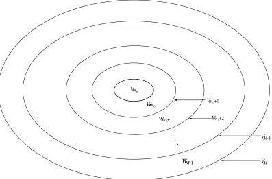
Throughout this thesis we denote the highest level of discretisation by M and NM will
denote the dimension of the space VM. Then, through recursive use of decomposition
(3.1.4), we can write the trial spaceVM as the sum of complement spaces
VM =Vm0
MM−1 m=m0
Wm, (3.1.9)
where m0 is some fixed coarsest level. This relationship is shown in Figure 3.1. Thus,
anyfM ∈VM can be expressed in single scale form, that is, with respect to the basisΦM,
as
fM =ΦTMαM, (3.1.10)
whereαM =hΦM, fi. We can also express the function in multiscale form, that is, with
respect to the basis
ΨM :=Φm0
M[−1 m=m0
Ψm, (3.1.11)
as
fM =ΦTm0αm0 +Ψ
T
m0βm0 +. . .+Ψ
T
M−1βM−1, (3.1.12)
whereβm =hΨm, fiform =m0, . . . , M −1. Since the sequenceV is dense inH, the
union
Ψ:=Φm0
∞
[
m=m0
Vm0
WM-1
VM-1
VM Wm
0
Vm 0+1
Vm0+2
Wm 0+1
. .
[image:35.612.129.526.59.320.2].
Figure 3.1: Decomposition ofVM into the complement spacesWm
is a candidate for a basis for the whole spaceH.
3.1.2
Vanishing Moments
An important property of wavelets is that of vanishing moments. A waveletψ has
vanish-ing moments of orderdif
Z
R
xiψ(x)dx = 0 fori= 0, . . . , d−1. (3.1.14)
It is the order of vanishing moments that governs the compression capacity of a wavelet.
Thus, for numerical applications we wish to have a high order of vanishing moments to
Example 3.1.1. (Haar Basis).
The simplest example of an orthogonal wavelet, is the Haar basis or Haar wavelets. Here,
H =L2[0,1]andVmis the space of piecewise constant functions with nodes atxi = 2im,
fori= 0,1, . . . ,2m
−1. Our scaling function is
φ(x) =
1 for 0≤x <1;
0 elsewhere.
(3.1.15)
Therefore, the countable setΦm ={φλ := 2
m
2φ(2m· −l)| λ = {m, l}, l ∈∆m}where ∆m ={0,1, . . . ,2m−1}is a basis for the spaceVm.
For the coarsest level m = m0 = 0, Φ0 = {φ} is a basis for the spaceV0. The space
V1 is the space of piecewise constant functions with nodes at0and 12. Therefore, Φ1 =
{φ1,0, φ1,1}is a basis for the spaceV1, where
φ1,0(x) =
√
2φ0,0(2x) for0≤x < 12;
0 otherwise,
(3.1.16)
φ1,1(x) =
√
2φ0,0(2x−1) for 12 ≤ x <1;
0 otherwise.
(3.1.17)
The Haar function or Haar wavelet is
ψ(x) =
1 for 0≤x < 12;
−1 for 12 ≤x <1;
0 elsewhere.
(3.1.18)
{ψλ := 2
m
2ψ(2m· −l)| λ={m, l}, l∈ ∇m}, where∇m ={0,1, . . . ,2m−1}, is a basis
for the spaceWm.
Since,V1 =W0⊕V0, we have two distinct bases for the spaceV1, namely,Φ1and{Ψ0∪
Φ0}. Therefore, a function in the spaceV1can be represented as a linear combination of
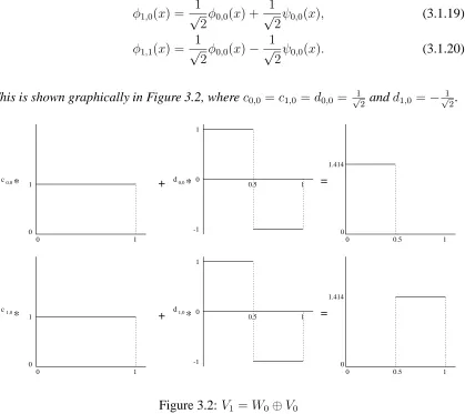
either the basisΦ1or the basis{Φ0∪Ψ0}. For the Haar basis it is easy to verify this,
φ1,0(x) =
1
√
2φ0,0(x) + 1
√
2ψ0,0(x), (3.1.19)
φ1,1(x) =
1
√
2φ0,0(x)− 1
√
2ψ0,0(x). (3.1.20)
This is shown graphically in Figure 3.2, wherec0,0 =c1,0 =d0,0 = √12 andd1,0 =−√12.
0
0 1
1.414
0.5 1
0 0 1
c0,0 d0,0
1
1 0.5
-1 0
* + * =
1 0
0 1
1
1 0.5
-1 0
c1,0 d1,0
0
0 1
1.414
0.5
[image:37.612.120.539.210.583.2]* + * =
3.1.3
Multiscale Transformations
The coefficient vectors αM and βm, for m = 0, . . . , M − 1, in (3.1.10) and (3.1.12),
respectively, convey different information. The coefficients αM in (3.1.10) indicate the
geometric location of the functionfM. However, the coefficientsβmrepresent the
differ-ence between the function representation at the current level and that of the previous level.
That is, the wavelets encode the detail information, or the correction that must be added
to the higher-level representation of a function. Therefore, we usually need all the entries
ofαM to obtain an accurate representation offM. However, many of the entries of βm
may be small and replacing such entries by zero may still permit a sufficiently accurate
approximation tofM. On the other hand, the pointwise evaluation offM is simpler in the
single scale form. Therefore to exploit the benefits of both representations, one needs a
method to convert one into the other.
Due to the nestedness of the spacesVmand the stability condition (3.1.3), everyφm,l ∈Vm
can be represented as an expansion of the functionsφm+1,i∈Vm+1. That is,
φm,l=
X
i∈∆m+1
ci,lφm+1,i, (3.1.21)
with a mask cml ={ci,l}i∈∆m+1 ∈ℓ2(∆m+1). Let Cm,0be the so-called refinement matrix
containing the cml as columns, then (3.1.21) can be rewritten as
ΦT
m =ΦTm+1Cm,0. (3.1.22)
functionsφm+1,i ∈Vm+1. That is,
ψm,l =
X
i∈∆m+1
di,lφm+1,i, (3.1.23)
with a mask dml = {di,l}i∈∆m+1 ∈ ℓ2(∆m+1). Let Cm,1 be the matrix containing the dml
as columns, then (3.1.23) can be rewritten as
ΨT
m =Φ
T
m+1Cm,1. (3.1.24)
Collectively (3.1.22) and (3.1.24) are known as the two scale relationships.
The decomposition Vm+1 = Vm ⊕ Wm is equivalent to the fact that the operator Cm :
ℓ2(∆m)×ℓ2(∇m)→ℓ2(∆m+1)is invertible, where
Cm := (Cm,1,Cm,0), (3.1.25)
and
Cm
βm αm
:=Cm,1βm+Cm,0αm, (3.1.26)
for αm ∈ ℓ2(∆m), βm ∈ ℓ2(∇m). Additionally the basis {Φm ∪Ψm}, of the space
Vm+1, is uniformly stable if and only if
kCmk=O(1),
C−m1=O(1), m→ ∞, (3.1.27) see [29].
For convenience, let Gm :=C−m1, where
Gm =
Gm,1
Gm,0
and
CmGm =Cm,1Gm,1+Cm,0Gm,0 =I. (3.1.29)
Therefore, the matrix Cm describes a change of basis for the spaceVm+1, from the basis
{Φm ∪ Ψm} to the basis Φm+1. The matrix Gm describes the reverse change. From
relationship (3.1.29) and the two scale relationships (3.1.22) and (3.1.24), we obtain the
reconstruction relationship
ΦTm+1 =ΦTmGm,0+ΨTmGm,1. (3.1.30)
Relationships (3.1.22), (3.1.24) and (3.1.30) are transformations that can be used to
con-vert the coefficients of (3.1.10) into the coefficients of (3.1.12) and vice versa. Let us now
derive these explicitly here. A functionfM ∈ VM can be expanded in single scale as in
(3.1.10), as well as in double scale form as
fM =ΦTM−1αM−1+ΨTM−1βM−1, (3.1.31)
with respect to the basis{ΦM−1∪ΨM−1}. Therefore, using (3.1.22) and (3.1.24), yields fM =ΦTM−1αM−1+ΨTM−1βM−1 =ΦTM CM−1,0αM−1+CM−1,1βM−1
. (3.1.32)
Comparing the r.h.s. of (3.1.32) with (3.1.10), we obtain
CM−1,0αM−1+CM−1,1βM−1 =αM. (3.1.33)
That is, the operator Cmapplied to the coefficients βαmm
produces the coefficientsαm+1.
Thus, repeated application of the operator Cm converts the coefficients of the multiscale
transformation
RM :βm0,M−1 →αM, (3.1.34)
where βm0,M−1 =
βM−1
.. .
βm0 αm0
. The transformation (3.1.34) is called the reconstruction
transformation, or reconstruction algorithm and is schematically given by
αM m 0 m 0,0 m 0,1 m 0+1 m
0 m0+1
m 0+1,0 m 0+1,1 m 0+2 m 0+2 M-1,0 M-1,1 M-1 ... ... β α C C α β C C α β C C β (3.1.35)
To express the transformation RM in matrix form, form < M, we define theNM ×NM
matrix
RM,m:=
I 0
0 Cm
, (3.1.36)
where I is the identity matrix of sizeNM−Nm+1. Then, the reconstruction transformation
RM in (3.1.34) can be written as
RM =RM,M−1· · ·RM,m0. (3.1.37)
The inverse transformation, transforms the single scale coefficientsαMoffM (see (3.1.10))
to the multiscale coefficients offM as in (3.1.12). Applying (3.1.30) tofM in single scale
form we obtain,
=ΦT
M−1(GM−1,0αM) +ΨTM−1(GM−1,1αM)
=ΦT
M−1αM−1+ΨTM−1βM−1. (3.1.38)
That is, the operatorGmapplied to the coefficientsαm+1results in the coefficients βαmm
.
Thus, repeated application of the operatorGmconverts the coefficients of the single scale
form of fM, (3.1.10), into the coefficients of the multiscale form (3.1.12), giving the
transformation
TM :αM →βm0,M−1. (3.1.39)
The inverse transformation (3.1.39) is called the decomposition transformation, or
decom-position algorithm and is schematically given by
m 0 m 0 M-1,0 M-1,1 M-1 M-1 M-2,0 M-2,1 M-2 M-2 m 0 m 0 α ... ... α α β α β M G G G G β G G ,1 ,0 (3.1.40)
Form < M, we define theNM ×NM matrix
TM,m:=
I 0
0 Gm
, (3.1.41)
where I is the identity matrix of sizeNM−Nm+1. Then, the decomposition transformation
TM in (3.1.39) can be written as
TM =TM,m0· · ·TM,M−1. (3.1.42)
(3.1.4). A constraint on the choice ofΨmis the stability of the multiscale transformations.
Theorem 3.1.1. ([30, Theorem 3.3]). The transformations RM and TM are well
condi-tioned in the sense that
kRMk,kTMk=O(1), M → ∞, (3.1.43)
if and only if the collectionΨof (3.1.13) is a Riesz basis ofH.
Example 3.1.2. Using the Haar basis of Example 3.1.1, we obtain the decomposition and
reconstruction algorithms for the Haar basis.
When we consider the Haar basis, the two scale relationships (3.1.22) and (3.1.24)
be-come
φλ =c0,0φm+1,2l(x) +c1,0φm+1,2l+1(x), (3.1.44)
ψλ =d0,0φm+1,2l(x) +d1,0φm+1,2l+1(x), (3.1.45)
for λ = {m, l}, m ∈ Z, l = 0, . . . ,2m −1. To find the coefficients c0,0 and c1,0, the
equidistant valuesx1 = 13 andx2 = 23 are substituted into relationship (3.1.44). Hence,
form = 0, we obtain the linear system
φ0,0
1 3
=c0,0φ1,0
1 3
+c1,0φ1,1
1 3
,
φ0,0
2 3
=c0,0φ1,0
2 3
+c1,0φ1,1
2 3
.
(3.1.46)
Solving (3.1.46), we findc0,0 = c1,0 = √12. Similarly, using relationship (3.1.45), we find d0,0 = √12 andd1,0 =−√12.
consider the projection coefficients off onto the spaceVm,
αλ =
Z
Iλ
f(x)φλ(x)dx
=c0,0
Z
Im+1,2l
f(x)φm+1,2l(x)dx+c1,0
Z
Im+1,2l+1
f(x)φm+1,2l+1 dx
=c0,0αm+1,2l+c1,0αm+1,2l+1, (3.1.47)
forλ ={m, l},m∈Z,l = 0, . . . ,2m−1. Similarly, the projection coefficients off onto
the spaceWm are
βλ =
Z
Iλ
f(x)ψλ(x)dx
=d0,0
Z
Im+1,2l
f(x)φm+1,2l(x)dx+d1,0
Z
Im+1,2l+1
f(x)φm+1,2l+1(x)dx
=d0,0αm+1,2l+d1,0αm+1,2l+1, (3.1.48)
forλ ={m, l}, m ∈ Z,l = 0, . . . ,2m−1. Relationships (3.1.47) and (3.1.48) together
are the decomposition algorithm in filter form for the Haar basis. In matrix form, for
M = 3, the decomposition algorithm isT3 =T3,0T3,1T3,2, where
T3,0 =
1 0 0 0 0 0 0 0
0 1 0 0 0 0 0 0
0 0 1 0 0 0 0 0
0 0 0 1 0 0 0 0
0 0 0 0 1 0 0 0
0 0 0 0 0 1 0 0
0 0 0 0 0 0 √1
2 −
1
√
2
0 0 0 0 0 0 √1
T3,1 =
1 0 0 0 0 0 0 0
0 1 0 0 0 0 0 0
0 0 1 0 0 0 0 0
0 0 0 1 0 0 0 0
0 0 0 0 √1
2 −
1
√
2 0 0
0 0 0 0 0 0 √1
2 −
1
√
2
0 0 0 0 √1 2
1
√
2 0 0
0 0 0 0 0 0 √1 2 1 √ 2
T3,2 =
1 √ 2 − 1 √
2 0 0 0 0 0 0
0 0 √1
2 −
1
√
2 0 0 0 0
0 0 0 0 √1
2 −
1
√
2 0 0
0 0 0 0 0 0 √1
2 − 1 √ 2 1 √ 2 1 √
2 0 0 0 0 0 0
0 0 √1
2 1
√
2 0 0 0 0
0 0 0 0 √1
2 1
√
2 0 0
0 0 0 0 0 0 √1
2 1 √ 2
We now derive the reconstruction algorithm for the Haar basis. Due to the decomposition
(3.1.4), a functionf ∈Vm+1 has two distinct representation, namely,
f(x) =
2m′−1
X
l′=0
αλ′φλ′(x), (3.1.49)
whereλ′ ={m′, l′}withl′ = 0, . . . ,2m′
−1, herem′ =m+ 1; and
f(x) =
2m−1
X
l=0
whereλ ={m, l}withl= 0, . . . ,2m
−1. Therefore, applying the two scale relationship,
(3.1.44) and (3.1.45), to equation (3.1.50), we obtain
f(x) =
2m
−1
X
l=0
(c0,0αλ +d0,0βλ)φm+1,2l(x) + (c1,0αλ +d1,0βλ)φm+1,2l+1(x). (3.1.51)
Then, comparing equations (3.1.49) and (3.1.51) we obtain the following reconstruction
algorithm, in filter form,
αm+1,2l =c0,0αλ +d0,0βλ
αm+1,2l+1 =c1,0αλ +d1,0βλ.
(3.1.52)
In matrix form, forM = 3, the reconstruction algorithm isR3 =R3,2R3,1R3,0, where
R3,2 =
1 √
2 0 0 0
1
√
2 0 0 0
−√1
2 0 0 0
1
√
2 0 0 0
0 √1
2 0 0 0
1
√
2 0 0
0 −√1
2 0 0 0
1
√
2 0 0
0 0 √1
2 0 0 0
1
√
2 0
0 0 −√1
2 0 0 0
1
√
2 0
0 0 0 √1
2 0 0 0
1
√
2
0 0 0 −√1
2 0 0 0
R3,1 =
1 0 0 0 0 0 0 0
0 1 0 0 0 0 0 0
0 0 1 0 0 0 0 0
0 0 0 1 0 0 0 0
0 0 0 0 √1
2 0
1
√
2 0
0 0 0 0 −√1
2 0
1
√
2 0
0 0 0 0 0 √1
2 0
1
√
2
0 0 0 0 0 −√1
2 0 1 √ 2
R3,0 =
1 0 0 0 0 0 0 0
0 1 0 0 0 0 0 0
0 0 1 0 0 0 0 0
0 0 0 1 0 0 0 0
0 0 0 0 1 0 0 0
0 0 0 0 0 1 0 0
0 0 0 0 0 0 √1
2 1
√
2
0 0 0 0 0 0 −√1
2 1 √ 2
To illustrate a use of the decomposition and reconstruction algorithms, we consider the
in multiscale form, that is, we use the basisΨ3. The resulting multiscale coefficients are β2,0 β2,1 β2,2 β2,3 β1,0 β1,1 β0,0 α0,0 =
0.131842719
0.3955448157
−0.1318482721
−0.3955448156
0.9003163161
−0.9003163163
0.6366197718
0 .
Therefore, applying the reconstruction algorithm to the multiscale coefficients, we obtain
the single scale coefficients,
R3
0.131842719
0.3955448157
−0.1318482721
−0.3955448156
0.9003163161
−0.9003163163
0.6366197718
0 =
0.7384680443
0.5820064299
0.0546133422
−0.5047715007
−0.7684680444
−0.5820064297
−0.0546133419
0.5047715010
.
Applying the decomposition algorithm to the single scale coefficients, we re-obtain the
multiscale coefficients.
The transformationsRM andTM in the present form are for theoretical analysis. In
prac-tice the matricesRM andTM are not computed, instead local filters are applied, see section
3.1.4
Wavelets on
[0
,
1]
The wavelets we have discussed so far are defined onR. However, we are concerned with
integral equations defined over a subset ofR. Therefore, we require wavelets defined on
a closed interval.
There are several methods which adapt wavelets defined onRto wavelets defined on an
interval; see [31, 32, 33, 34]. Here, following Daubechies [26], we briefly introduce two
methods for defining wavelets on the interval[0,1]. The first and most basic method is to
use wavelets defined overR, with the functionfset to zero outside of[0,1]. However, this
method introduces a discontinuity in the function at the interval’s boundary. This leads
to large wavelet coefficients for wavelets whose support overlaps the interval’s boundary.
Furthermore, this method is not computationally efficient.
The second method is the so-called periodized wavelets. We start with the scaling function
φ and the waveletψ defined overR. For m = 0,1, . . ., we define the periodized scaling
function and wavelet as
φperλ (x) = X
i∈∆m
φλ(x+i) = 2
m
2 X
i∈∆m
φ(2mx
−2mi
−l), (3.1.53)
forλ ={m, l},l ∈∆m and
ψλper(x) = X
i∈∇m
ψλ(x+i) = 2
m
2 X
i∈∇m
ψ(2mx−2mi−l), (3.1.54)
forλ = {m, l},l ∈ ∇m. Here,∆m = ∇m =Z. Clearly, bothφperλ andψ
per
λ are periodic
of period 1. The spacesVper
m andWmperare defined as
Vper
m := span{φ
per
and
Wmper := span{ψ
per
λ | λ={m, l}, l ∈Z}, (3.1.56)
respectively.
Since the scaling function and wavelet are periodic with period 1, φperm,l+2m = φ per
m,l and
ψm,l+2per m = ψ per
m,l, the spaces Vmper andWmper are 2m-dimensional spaces, [26, 23]. These
spaces inherit the multiresolution properties of the non-periodized spaces Vm and Wm.
That is,
V0per ⊂V1per ⊂. . .⊂L2[0,1], (3.1.57)
∞
[
m=0
Vmper =L2[0,1] (3.1.58)
and
Vper
m =V
per
m−1⊕W
per
m−1. (3.1.59)
In the remaining section of this chapter we discuss the bases we use in this thesis, namely,
the multiwavelets. These are a wavelet basis developed for the interval[0,1].
3.2
Multiwavelets on
[0
,
1]
Wavelets are attractive for the numerical solution of integral equations, because their
van-ishing moments property leads to operator compression [21, 35]. However, to obtain
wavelets with compact support and high order of vanishing moments, the length of the
support increases as the order of the vanishing moments increases, [26, 36]. This causes