Ranking genes with respect to differential expression

Deposited research article

Ranking genes with respect to differential expression

Per Broberg

Address: Molecular Sciences, AstraZeneca R&D Lund, S-221 87 Lund, Sweden

Correspondence: Per Broberg. E-mail: [email protected]

comment

reviews

reports

deposited research

interactions

information

refereed research

.deposited research

AS A SERVICE TO THE RESEARCH COMMUNITY, GENOME BIOLOGY PROVIDES A 'PREPRINT' DEPOSITORY

TO WHICH ANY ORIGINAL RESEARCH CAN BE SUBMITTED AND WHICH ALL INDIVIDUALS CAN ACCESS

FREE OF CHARGE. ANY ARTICLE CAN BE SUBMITTED BY AUTHORS, WHO HAVE SOLE RESPONSIBILITY FOR

THE ARTICLE'S CONTENT. THE ONLY SCREENING IS TO ENSURE RELEVANCE OF THE PREPRINT TO

GENOME BIOLOGY'S SCOPE AND TO AVOID ABUSIVE, LIBELLOUS OR INDECENT ARTICLES. ARTICLES IN THIS SECTION OF

THE JOURNAL HAVE NOTBEEN PEER-REVIEWED. EACH PREPRINT HAS A PERMANENT URL, BY WHICH IT CAN BE CITED.

RESEARCH SUBMITTED TO THE PREPRINT DEPOSITORY MAY BE SIMULTANEOUSLY OR SUBSEQUENTLY SUBMITTED TO

GENOME BIOLOGY OR ANY OTHER PUBLICATION FOR PEER REVIEW; THE ONLY REQUIREMENT IS AN EXPLICIT CITATION

OF, AND LINK TO, THE PREPRINT IN ANY VERSION OF THE ARTICLE THAT IS EVENTUALLY PUBLISHED. IF POSSIBLE, GENOME

BIOLOGYWILL PROVIDE A RECIPROCAL LINK FROM THE PREPRINT TO THE PUBLISHED ARTICLE. Posted: 5 August 2002

Genome Biology 2002, 3(9):preprint0007.1-0007.23

The electronic version of this article is the complete one and can be found online at http://genomebiology.com/2002/3/9/preprint/0007

© BioMed Central Ltd (Print ISSN 1465-6906; Online ISSN 1465-6914)

Received: 31 July 2002

This is the first version of this article to be made available publicly.

Ranking genes with respect to differential expression

Per Broberg

Molecular Sciences, AstraZeneca R&D Lund, S-221 87 Lund, Sweden Correspondence: [email protected]

Abstract

Background

In the pharmaceutical industry and in academia substantial efforts are made to make the best use of the promising microarray technology. The data generated by

microarrays are more complex than most other biological data attracting much attention at this point. A method for finding an optimal test statistic with which to rank genes with respect to differential expression is outlined and tested. At the heart of the method lies an estimate of the false negative and false positive rates. Both investing in false positives and missing true positives lead to a waste of resources. The procedure sets out to minimise these errors. For calculation of the false positive and negative rates a simulation procedure is invoked.

Results

The method outperforms commonly used alternatives when applied to simulated data modelled after real cDNA array data as well as when applied to real oligonucleotide array data. In both cases the method comes out as the over-all winner. The

simulated data are analysed both exponentiated and on the original scale, thus providing evidence of the ability to cope with normal and lognormal distributions. In the case of the real life data it is shown that the proposed method will tend to push the differentially expressed genes higher up on a test statistic based ranking list than the competitors.

Conclusions

The approach of making use of information concerning both the false positive and false negative rates in the inference adds a useful tool to the toolbox available to scientists in functional genomics.

Background

The microarray technology has revolutionized modern biological research by permitting the simultaneous study of a great part of the genome. The blessings stemming from this also brings the curse of high dimensionality of the data output. Microarrays play an important role in finding drug targets. This application provides the primary practical motivation for the method presented.

eligible genes considerably. Furthermore, the fact that a group of genes in the same functional class show evidence of differential expression

may be much more telling than the individual p-values as such. However the rank order does play a role: It is generally sensible to validate a target in the drugable class with a smaller p -value prior to proceeding to one with a larger p -value. Sometimes it is possible to be guided by the performance of known drug targets in the choice of cut-off, but at any rate p -values have the greatest impact on decisions by providing a preliminary ranking of the genes. This is not to say that one should never take multiplicity into account or that this method in some way replaces correction for multiplicity. On the contrary samroc provides the basis for such calculations, see Section Samroc.

The approach presented could be applied to different types of test statistics, but to fix ideas one particular type recently proposed will be used. In the [2] a methodology based on a regularised t-statistic is described:

S

S

diff

d

+

=

where diff is an effect estimate, e.g. a group mean difference, S is a standard error, and S0 is the regularising constant. This formulation is quite general and e.g. includes the estimation of a contrast in an ANOVA. Putting S0=0 will yield a t-statistic. The constant is found by removing the trend in d as a function of S in moving windows across the data. The technical details are spelled out in [3]. The statistic calculated this way will be referred to as SAM.

The basic idea with d is to eliminate some false positives with low values on S. It seems more relevant to optimise with respect to what is really the issue, namely the false positive and false negative rates. This is the intuition behind the approach.

An alternative to the statistic (1) is d= diff/√(S02+S2), or d= diff/√(wS02+(1-w)S2) for some weight w, which is basically the statistic proposed in [4]. Its performance appears to be very similar to that of (1) (data not shown). A more imaginative, but rather unorthodox, approach to comparing two groups would be to use m=Σe-aXi/n, where Xi is assumed positive, for a fold change calculation of the measures m1 and m2 for the two groups: MG=max{ m1, m2 }/min{ m1, m2}. The statistic m estimates the moment generating function. The case a= 1 will be evaluated.

In this article another goodness criterion is proposed and argued. What is really relevant in choosing a good method is choosing one with an attractive Receiver Operating Characteristics (ROC) curve. By an attractive ROC curve is meant a plot of Proportion False Positives against Proportion False Negative that is as close to the axes as possible. This will minimise the number of genes that are falsely declared positive and falsely declared negative for a given significance level α and value on

S0. It will also minimise the distance to the origin, which will be the criterion for finding an optimal value on S0 as well as on α, see Fig. 2.

The structure of the article is the following. First the criterion is explained in detail. Then the estimation problems concerning the false positive and false negative rates are solved. Finally, the algorithm is outlined and tested on some simulated and some real data.

Methods

The criterion

A comparison of methods in terms of their ROC curves is displayed in Figure 4 of [1]. There a method whose ROC curve lies below another one is preferred, see Figure 2. If we agree that it be sensible to compare methods with respect to their ROC curves, then estimation procedures ought to find parameter estimates that make the ROC curve optimal in some sense. This section suggests a goodness criterion for the ROC curve.

By False Discovery Rate (FDR) we mean the proportion of false positives among the significant genes, seer e.g. [2]. Multiplying FDR by the proportion of genes that are declared significant and dividing by the number of genes we

obtain the False Positive rate (

FP

Assume that we can, for given significance level α, estimate FP(α) and FN(α), and let

h be a spline approximating the regression of FP on FN. Let us require that FP is less than or equal to FPmax, and likewise FN less than or equal to FNmax. Furthermore, put h1(x)=min{h(x), FPmax}. The goodness criterion is then formulated in terms of the distance of points on the curve h1 to the origin, which in mathematical symbols may be put as

( )

{

}

C _{x FP} 2 ₁2

max

min +

= _≤ (2)

Given a value on S0 a set of (FP(α), FN(α)) will come out, and from this a spline h is given. Finally, calculate the criterion (2). Repeat the procedure for a number of S0 and α values and choose the combination with the smallest distance.

If one has an assessment regarding the relative importance of FP and FN, that may be reflected in a version of the criterion (2) that incorporates

weights.

Estimating FP

Using the permutation method to simulate the null distribution of no change we can obtain a p-value for a two-sided test, as detailed below.

The data matrix has genes in rows and arrays in columns. Let d(j)*k be the value of the jth gene statistic in the kth permutation of columns and the p-value for gene i

equals

( )

( )

( )

{

}

where M is the number of genes, d(i) the observed statistic for gene i, and B the number of permutations [2, 10, 11].

Thus given the significance level α the genes considered as differentially expressed will have the proportion given by

( ) {

}

M

P

i

p

α

=

#

:

≤

α

(4)

, where ‘#’ denotes the cardinality of the set.

According to [12] FDR ≤ α / p(α); equality is assumed in their treatment.

Furthermore, there is a bound by Benjamini and Hochberg [13] that states that FDR ≤ M x P(i)/i, where P(i) is the largest ordered p-value which is declared significant. In terms of the entities above we have i= p(α) x M and P(i)=maxi {Pi: Pi≤α}. Since P(i) is the largest p-value called significant, we have P(i) ≤α. In [14] the estimate FDR=p0 x P(i) / p(α) is derived, where p0 is the proportion unchanged genes. This suggests that the bound

( )

p

( )

α

p

α

p

( )

α

P

p

FDR

≈

ˆ

×

/

≤

ˆ

×

/

could be used as a reasonable approximation of FDR.

The current version of samroc uses the estimate

( )

{

}

2

/

:

#

ˆ

0

M

q

i

d

q

i

p

=

≤

≤

where qX is the X% fractile of the d*, cf. [3]. This estimate makes use of the fact that the genes whose test statistics fall in the quartile range will be predominantly the unchanged ones. More material on this matter follows in the Appendix.

( )

p

FP= ₂₂ =

α

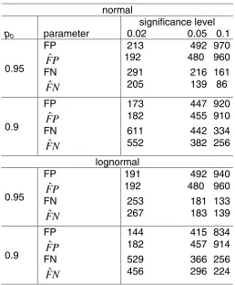
Although not perfect the estimate of FP will tend to follow the change in true FP quite well, see Table 2.

Estimating FN

One way to attack the problem of estimating FN would be the following.

By definition the proportion false negative consists of all genes minus the true negative and the positive.

Using the notation in Table 1 FN= p21. From this, we may proceed to p0=p11+p22. Furthermore, p(α) = p12+p22 and p2 2= FP. Thus

p11 = p0-p22. Finally p21 is identified from p21 = 1 - p11 - p 12 - p22.

Using (5) one obtains

(

α

) ( )

p

α

p

p

FN

=

=

1

−

ˆ

1

−

−

The graph we want to study is the one of the estimate

(

α

) ( )

p

α

p

FN

=

1

−

ˆ

1

−

−

versus the estimate of

( )

FP=

α

The Samroc algorithm

The statistic (1) calculated in the following way will be referred to as samroc, and comes with SAG 0.9-13.

Before the algorithm starts the S’s are smoothed as a function of the average expression level of the gene, if the option smooth = T . By default smooth = F.

The algorithm suggested can be summarised by the following steps

1. Calculate the effect estimate, e.g. difference between group means 2. Calculate the standard errors

3. Generate effect estimates under the null hypothesis, through B permutations (by default B = 100).

4. Calculate standard errors for these simulation estimates

6. Iterate over new values of S0, i.e. a number of fractiles of S, and a number of

α’s to find an optimum.

Samroc also outputs a suggested significance level as well as an optimal S0, that is estimated to minimise the criterion (1). Furthermore, the function outputs the

observed test statistic, the simulation test statistic and the uncorrected p-values. Thus, one may use this output to calculate corrected p-values, e.g. by using the package multtest [15] to obtain the multiple test procedure detailed in [10] (see also [16]), or samfdr in SAG to obtain the decisions based on the FDR [2]. Additionally, the R base package offers the function p.adjust, which provides the multiple test options Bonferroni, Holm and Hochberg.

Since the p-values they produce are monotone in the uncorrected ones they gives genes the same rank order as the uncorrected p-values. One shall bear in mind that the multiple test procedures tend to be very strict, and thus provide low power for detecting changed genes. New and promising ideas based on the FDR concerning how to increase power exist, e.g. [14]. The subject is important and complex, and would easily fill up an article this size.

A modified algorithm which starts by fixing the number of genes to be selected will be evaluated in the future.

Results

When testing methods in this field it is difficult to find suitable data where something is known about true status of the genes. If one chooses to simulate, then the distributions may not be entirely representative of a real life situation.

If can find non-proprietary real life data, then the knowledge as to which genes are truly changed may be uncertain. The bulk of my experience with this method comes from analysing proprietary data from experiments run on the Affymetrix U95

GeneChips. I have had very good results, but my telling so will not convince the critical mind, so I have tried to find both relevant simulation models and relevant publicly available real life data.

It has been common to simulate data, as in [4, 1, 14]. All these use normal distributions, in the case of [1] conditional normal distributions.

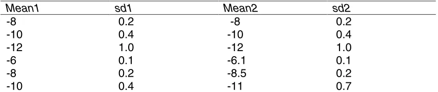
The data used in this article were simulated using mixtures of the distributions described in [4]. These theoretical distributions were modelled after the real E.coli cDNA data presented in [17]. To make the situation a little more realistic the distributions of the changed genes are now chosen randomly among the three last bottom rows of Table 3. The null distribution was obtained by mixing the distributions in the first three rows of Table 3. The simulation program, including the seed, is available at the supplementary web site [7].

In the comparison samroc, t-test, Wilcoxon, MG, Fold Change, the Bayesian method in [1], and SAM [2] were competing. By the t-test we mean the unequal variance t -test: t= (mean1-mean2)/√(s12/n1+s22/n2) for sample means mean1 and mean2 and sample variances s12, s22. The Wilcoxon rank sum test is based on the sum Ws of the ranks of the observations in one of the groups Ws=R1…+Rn1 [18]. The Bayesian method calculates the posterior odds for genes being changed (available as functions stat.bay.est in the R package SAG, and stat.bayesian in sma ([1],[5]). Finally, Fold Change equals FC = max{mean1, mean2}/min{mean1, mean2}.

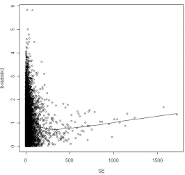
The t-test is known to have an important optimality feature called Uniformly Most Powerful unbiased when data are normal [19]. Basically, this means that the t-test is hard to beat when data are normal. However, when the number of observations is low the estimate of the standard error (SE) which goes into the

denominator can sometimes play tricks. When the SE is low there is an increased risk of obtaining false positives as has been noted by several authors. This problem predominantly appears at low expression levels.

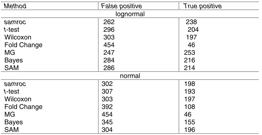
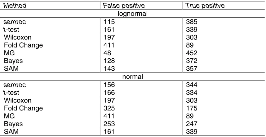
Let us start by the simulated data that is expected to contain 5% changed genes, see Table 4. When data are truly normal and there are as many as 4 observations

per group samroc performs best, followed by SAM together with Wilcoxon, and the MG method last, being a total disaster. The program estimates p0 at 96%, the regularising constant S0 is set to 0, and the suggested cut-off is 0.02.

When the same data is exponentiated, thus giving lognormal distributions, MG

comes out first, followed by samroc, the t-test and Wilcoxon lag far behind, and Fold Change is clearly a failure. This time p0 is estimated at 96%, S0 is taken to be the minimum S, and the suggested cut-off is 0.02.

When data are normal and the expected proportion of changed genes equals 10%,

p0 is estimated at 91%, 0 is chosen as the value of S0, the suggested cut-off is 0.03. Now samroc comes out on top, followed by SAM and the t-test, and again MG cannot cope with normal data, see Table 5.

These data were also exponentiated and p0 was then estimated at 91%, and S0 was chosen to be the minimum of the S’s, while the cut-off was set to 0.03. The MG method came out a clear winner, followed by samroc and Bayes, and Fold Change trailing behind.

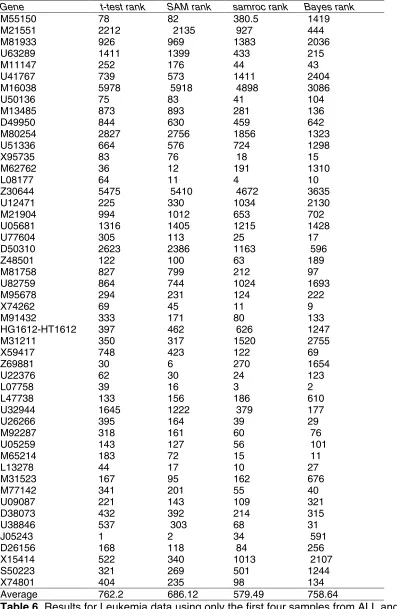
Next let us look at the leukaemia data from [20] which consists of 38 samples run on the Affymetrix Hu6800FL oligonucleotide chip. The Average Difference values on 7129 probe sets were downloaded from [21]. The samples either belong to the acute myeloid leukaemia (ALL) or the acute lymphoblastic leukaemia (AML) category, with 27 replicates of the first category and 11 of the second. A review of how three methods fare with these data is presented in [22]. In that reference 50 genes are listed that based on statistical analysis of the full set of 38 samples and on biological evidence are believed to be differentially expressed when comparing ALL to AML. With the full sample the results agree well between methods, and there is reason to believe that the genes are truly differentially expressed. With a large sample size, the choice of method is not so critical as with a small. However, a good method would pick out these genes already at a smaller sample size. Therefore, it is reasonable to score the methods by the average rank of the genes on the list.

current treatise, where the relative merits of the methods for ranking genes is the issue.

In Table 6 we can see the ranks of the genes among all genes. In the first two columns we see the t-test and SAM, and it is evident that they agree quite well on most genes, which is not so surprising, since SAM is a slightly modified t-test. Looking at the over-all average ranks in the bottom row reveals that samroc tends to push the differentially expressed genes higher up the list than the other methods. Though its apparent similarity to SAM, samroc has a different behaviour. The Bayes method may have some problems caused by the assumption of conditional normality at this sample size with these data.

Discussion

Whether to look at data on a log scale or not is a tricky question, and is beyond the scope of this article. However, from the above it is appears that the best performance by the tests considered is achieved when data are lognormal. But the methods are tested on normal, lognormal and real life data, in order to supply a varied testing ground.

The proposed method comes out better than the original SAM statistic in every test performed. Obviously, the ordinary Fold Change is a disaster, as has been noted by several authors before. The success of MG is rather unexpected and hard to

understand, and on top of that the statistic corresponds to a very general hypothesis. But the fact remains that it is a tough contender when data are close to lognormal, which is often the case. In contrast to samroc, however, it suffers from being highly sensitive to distributional assumptions. Maybe a calibration of a using the algorithm outlined in this article can further extend its use. The samroc statistic d is robust and flexible in that it can address all sorts of problems that suit a linear model.

The methodology adjusts the regularising constant when data are non-normal and achieves an improved performance. The algorithm ranks the genes in a reliable fashion, and also gives some rough idea of how many genes it makes sense to look closer at.

A typical run with real life data will take several hours on a desktop computer. To make this methodology better suited for production it would be a good investment to translate part of the R code, or the whole of it, into C.

In order to improve on standard univariate tests one must make use of the fact that data are available on a large number of related tests. In this article

it has been shown one way of achieving this goal. The conclusion is that it is possible and sensible to calibrate the test with respect to estimates of the false positive and false negative rates.

Acknowledgement

Ingrid Lonnstedt generously made the code to a linear models version of stat.bay.est

available. Furthermore, the comments from Terry Speed are gratefully acknowledged.

References

2. Tusher V.G., Tibshirani R., Chu G: Significance analysis of microarrays applied to the ionizing radiation response.Proc. Natl. Acad. Sci.USA 2001, 98:

5116-5121

3. Chu G, Narasimhan B, Tibshirani R, Tusher, VG: SAM Version 1.12

"Significance Analysis of Microarrays" User’s Guide and technical document,

2001

4. Baldi P, Long AD : A Bayesian Framework for the Analysis of Microarray Expression Data: Regularized t-Test and Statistical

Inferences of Gene Changes. Bioinformatics 2001, 17: 509-519

5. The R project

[www.cran.r-project.org]

6. Ihaka R, Gentleman R: (1996) R: A language for data analysis and graphics.

Journal of Computational and Graphical Statistics 1996,5: 299-314

7. Supplementary web page

[http://home.swipnet.se/pibroberg]

8. Lovell DR, Dance CR, Niranjan M, Prager RW, Dalton KJ: Ranking the effect of different features on the classification of discrete valued data, in Engineering Applications of Neural Networks 1996, (Kingston on Thames, London), pp. 487-494

9. Genovese C, Wasserman L: Operating Characteristics of the FDR procedure., technical report Carnegie Mellon University 2001.

10. Dudoit S,Yang YH, Speed TP, Callow MJ: Statistical methods for identifying differentially expressed genes in replicated cDNA microarray experiments.,

Statistica Sinica 2002, 12: 111-140

11. Davison AC, Hinkley DV Bootstrap Methods and their Application. Cambridge : Cambridge Univeristy Press, 1997

12. Efron B, Tibshirani R, Storey JD, Tusher VG: Empirical Bayes analysis of a microarray experiment.Journal of the American Statistical Association 2001,96:

1151-1160

13. Benjamini Y, HochbergY: (1995) Controlling the false discovery rate :

a practical and powerful approach to multiple testing. J.R. Statist. Soc. B. 1995,

57: 963-971.

14. Storey JD: (2001) A Direct Approach to False Discovery Rates.technical report Stanford 2001

15. Bioconductor software for bioinformatics

[http://www.bioconductor.org]

16. Callow M J, Dudoit S , Gong EL , Speed TP, Rubin EM : Microarray

17. Arfin SM, Long AD, Ito T, Tolleri L, Riehle MM, Paegle ES, Hatfield GW : Global gene expression profiling in escherichia coli K12: the effect of integration host factor.J. Biol. Chem. 2000, 275: 29672-29684.

18. Lehmann EL: Nonparametrics :Statistical Methods based on Ranks. San Francisco, Holden-Day, 1975

19. Lehmann EL: Testing Statistical Hypothesis. New York: Wiley, 1959

20. Golub TR, Slonim DK, Tamayo P, Huard C, Gaasenbeek M, Mesirov JP, Coller H, Loh ML, Downing JR, Caligiuri MA et al.:Molecular classification of

cancer:class discovery and class prediction by gene expression monitoring.

Science 1999, 285: 531-537

21. Dataset used in [20]

[http://www-genome.wi.mit.edu/cgi-bin/cancer/datasets.cgi]

22. Pan W: (2002) A comparative review of statistical methods for discovering differentially expressed genes in replicated microarray experiments.

Bioinformatics 2002, 18: 456-554.

23. Irizarry RA, Hobbs B, Speed TP: (2001) Exploration, Normalization, and

Summaries of High Density Oligonucleotide Array Probe Level Data. Manuscript in preparation, available at

http://www.stat.berkeley.edu/users/terry/zarray/Affy/GL_Workshop/genelogic2001.ht ml

Figure 1. Often with real microarray data the absolute value of the t-statistic is a function of the standard error SE, and there is an erratic behaviour of the statistic for small values of SE with an increased risk of false positives. By choosing the constant

0.0 0.2 0.4 0.6 0.8

0.

0

0.

2

0.

4

0.

6

0.

8

False Positive rate

F

a

ls

e

N

e

g

a

ti

v

e

r

a

te

−6

−4

−2

0

2

4

−4

−2

0

2

4

d(i)

Expected order statistic

0.40

0.45

0.50

0.55

0.60

0.65

0.70

0.030

0.040

0.050

Cut−off

Figure 3. A subset of the data from Golub et al consisting of the first four samples from each group, was used to assess the performance of the t-test, SAM, samroc

and the Bayesian method. The upper panel shows the ordered observed d-statistics versus the expected ordered statistics calculated from the simulation. Looking at the graph it appears that rather a lot of genes are changed. The lower panel shows the estimated FDR as a function of the cut-off δ, such that genes with |d-dexpected| >δ will be called differentially expressed. Choosing a cut-off of 0.7, i.e. calling genes that fulfill |d-dexpected| > 0.7 differentially expressed will only give about 3% false positives. The proportion of unchanged genes is estimated at 84%, and S0 in (1) is put to the

Tables

Negative Positive

True p11 p12 T

False p21 p22 F

N P 1

normal

significance level

p0 parameter 0.02 0.05 0.1

FP 213 492 970

P

F

ˆ

FN 291 216 161

0.95

N

Fˆ 205 139 86

FP 173 447 920

P

F

ˆ

FN 611 442 334

0.9

N

Fˆ 552 382 256

lognormal

FP 191 492 940

P

F

ˆ

FN 253 181 133

0.95

N

Fˆ 267 183 139

FP 144 415 834

P

F

ˆ

FN 529 366 256

0.9

N

Fˆ 456 296 224

Table 2. The actual and estimated FP’s and FN’s for the simulated data in the Results section. Often FP is quite well estimated, while

Mean1 sd1 Mean2 sd2

-8 0.2 -8 0.2

-10 0.4 -10 0.4

-12 1.0 -12 1.0

-6 0.1 -6.1 0.1

-8 0.2 -8.5 0.2

-10 0.4 -11 0.7

Method False positive True positive

lognormal

samroc 262 238

t-test 296 204

Wilcoxon 303 197

Fold Change 454 46

MG 247 253

Bayes 284 216

SAM 286 214

normal

samroc 302 198

t-test 307 193

Wilcoxon 303 197

Fold Change 392 108

MG 454 46

Bayes 345 155

SAM 304 196

Table 4. Genes were ranked with the statistical methods in terms of degree of

Method False positive True positive

lognormal

samroc 115 385

t-test 161 339

Wilcoxon 197 303

Fold Change 411 89

MG 48 452

Bayes 128 372

SAM 143 357

normal

samroc 156 344

t-test 166 334

Wilcoxon 197 303

Fold Change 325 175

MG 411 89

Bayes 253 247

SAM 161 339

Gene t-test rank SAM rank samroc rank Bayes rank

M55150 78 82 380.5 1419

M21551 2212 2135 927 444

M81933 926 969 1383 2036

U63289 1411 1399 433 215

M11147 252 176 44 43

U41767 739 573 1411 2404

M16038 5978 5918 4898 3086

U50136 75 83 41 104

M13485 873 893 281 136

D49950 844 630 459 642

M80254 2827 2756 1856 1323

U51336 664 576 724 1298

X95735 83 76 18 15

M62762 36 12 191 1310

L08177 64 11 4 10

Z30644 5475 5410 4672 3635

U12471 225 330 1034 2130

M21904 994 1012 653 702

U05681 1316 1405 1215 1428

U77604 305 113 25 17

D50310 2623 2386 1163 596

Z48501 122 100 63 189

M81758 827 799 212 97

U82759 864 744 1024 1693

M95678 294 231 124 222

X74262 69 45 11 9

M91432 333 171 80 133

HG1612-HT1612 397 462 626 1247

M31211 350 317 1520 2755

X59417 748 423 122 69

Z69881 30 6 270 1654

U22376 62 30 24 123

L07758 39 16 3 2

L47738 133 156 186 610

U32944 1645 1222 379 177

U26266 395 164 39 29

M92287 318 161 60 76

U05259 143 127 56 101

M65214 183 72 15 11

L13278 44 17 10 27

M31523 167 95 162 676

M77142 341 201 55 40

U09087 221 143 109 321

D38073 432 392 214 315

U38846 537 303 68 31

J05243 1 2 34 591

D26156 168 118 84 256

X15414 522 340 1013 2107

S50223 321 269 501 1244

X74801 404 235 98 134

Average 762.2 686.12 579.49 758.64

Appendix

Estimation of p0

Using the model in [12] where the distribution is assumed to be a mixture of

differentially expressed genes (denoted 1) and rest (denoted 0), such that in terms of densities f(x)=p1 f1(x)+(1- p1) f0(x), the entries of Table 1 may be estimated given a value on p1 . Let p0 = 1- p1, which is not identifiable without strong parametric assumptions. There exist however a number of suggested solutions.

From the relation (3.9) in [12] p1≥ 1 – min{f0 / f}. Similarly one may show that p1 ≤ f(z) / f1(z) = p1*/(1-p0*f0(z)/f(z)), taking p0* and p1* from the previous relation. The right members of the two previous relations may be estimated by a bootstrap explained in the reference. This procedure basically uses the data and the bootstrapped data to estimate the log odds for having an observation of one type versus the other in an interval and smoothes the log-odds as a function of the test statistic with a spline. A third way to estimate p0 is to use the assumption that the expected difference under the null hypothesis is zero E0[d] = 0, and a variance decomposition. From E[d] = µ = p1µ1 and the variance decomposition σ2 =Var[d]= p1 (µ1 -µ)2 + p0 µ2 + p1σ12+ p0 σ02, we have, disregarding p1σ12 and using µ1 = µ / p1, the inequality σ2 ≥ p0 {µ2(p0/ p1 + 1)+ σ02}. The moments are estimated from the sample and the bootstrap, and by assuming equality, and thereby inflating p0 a bit, we can solve for p0. Assuming equality in the first of the two previous inequalities, using the result in the second and assuming equality also there, and taking the mean of the three estimates,

In a short series of simulation tests the estimate (3) performed best. But other options will be considered in preparation for the next release

of samroc.

Why it is not enough to control FDR

If one agrees that, in the notation of Table 1, it is desirable to minimise the proportion of incorrectly called genes p12+p21 (or in general some increasing function of these), then it will not suffice to minimise FDR. The FDR ≈ p0 x α / p(α), with α the

better to balance FDR and power by using the information on p21 and p12 that we