Conference proceedings 2010

(1)

Conference proceedings 2010

SPARC,

Title

Conference proceedings 2010

Authors

SPARC,

Type

Conference or Workshop Item

URL

This version is available at: http://usir.salford.ac.uk/16822/

Published Date

2010

USIR is a digital collection of the research output of the University of Salford. Where copyright

permits, full text material held in the repository is made freely available online and can be read,

downloaded and copied for noncommercial private study or research purposes. Please check the

manuscript for any further copyright restrictions.

(2)

Proceedings of the

Salford Postgraduate Annual

Research Conference

(SPARC)

2010

(3)

Proceedings of the Salford Postgraduate Annual Research Conference (SPARC) 2010

Published by

The University of Salford Salford

Greater Manchester M5 4WT

(4)

Preface

Postgraduate research is the dynamo that drives innovative new work at good universities, and we are particularly proud of the work of our postgraduate students. SPARC brings together the best of this research across key fields that well express our university’s strong themes of enquiry. The annual SPARC conference provides a dynamic forum for research students and supervisors to present and discuss new knowledge, fostering connections across disciplines that will open up areas for the future.

Professor Martin Hall

Vice-Chancellor, University of Salford

Welcome to the 2010 proceedings of the Salford Postgraduate Annual Research Conference (SPARC). This selection of papers provides an excellent indication of the scope and scale of the two day interdisciplinary conference, and testifies to the quality and intellectual rigour of the research projects showcased there.

One of the defining characteristics of SPARC is its openness to all disciplines and research topics. This enables the participants to set the priorities of the conference, and allows for natural themes to emerge. This broad-ranging selection of thirty papers spans a wealth of disciplines – from life sciences, management, finance, computing, education, and the built environment through to sociology, art and literature studies. This publication offers a snapshot of that range: alongside Salford’s researchers, there are contributions from postgraduates at the Universities of Liverpool John Moores, Exeter, Bolton University, Cardiff University, Suffolk and Limerick Institute of Technology in Ireland.

As well as facilitating conversations between disciplines, SPARC offers space for informal and academic networking between researchers from different universities, with presenters drawn from different regions of the UK and internationally. Providing an environment for cross - institutional engagement is just one of the ways in which the annual conference supports researcher development. It is an opportunity to develop individual research projects, giving presenters the chance to test out ideas on new audiences, receive valuable feedback from the academic community, make their work known and consequently raise their research profile. At the same time, the conference is also about professional development – allowing early career academics to develop all important conference presentation skills, to practise the art of translating complex research ideas into a clear and concise format, and to communicate those ideas to audiences outside of their immediate specialism. This has valuable implications in terms of employability, encouraging the development of the kind of transferable skills that researchers are increasingly expected to demonstrate.

(5)

access ethos of the unrestricted sharing of knowledge is very much in keeping with the spirit of the conference.

If you would like to find out more information about the annual conference and details other support for early career researchers offered by Salford’s Graduate Studies team, please visit our website at http://www.pg.salford.ac.uk

Dr Victoria Sheppard Dr Sonja Tomaskovic

(6)

Evaluation of Car-following Models Using Field Data

Hamid A.E. Al-Jameel, University of Salford

Abstract

Traffic congestion problems have been recognised as a serious problem in all large urban areas. It can

significantly reduce urban mobility. Therefore, it has become a major concern to the transportation and

business communities and to the public in general. Different techniques have been proposed to alleviate

this problem. One of these techniques is a traffic simulation. It has been used effectively as it can

represent real life, to some extent, and apply different strategies without the need to make physical

changes. Car-following models represent the basic unit that governs the longitudinal movement for each

traffic simulation model. The efficiency of a traffic simulation model mainly depends on its core units:

car-following and lane changing.

In this study, three car-following models (namely, CARSIM, WEAVSIM and PARAMICS) were tested.

The first two of these models were rebuilt using Visual Compact FORTRAN Version-6.5. The models

were tested using three different sets of data from single lane traffic. These sets of data have been

collected using two different methods of collecting data from three regions. In addition, different traffic

conditions have been included in this data such as high speed, low speed and “stop and go conditions”.

The results indicated that CARSIM gave the most accurate representation of real life situations.

Therefore, the assumptions of this model were adopted in a newly developed model to represent traffic

behaviour in weaving sections to evaluate the factors affecting the weaving capacity.

Keywords:

Traffic micro-simulation, car-following model, CARSIM and WEAVSIM

1. Introduction

Traffic congestion problems have been recognised as a serious problem in all large urban areas. It can

significantly reduce urban mobility. Therefore, it has become a major concern to the transportation and

business communities and to the public in general. Different techniques have been proposed to alleviate

(10)

represent real life, to some extent, and applies different strategies without the need to make physical

change on site before implementing such strategies. Car-following model represents the basic unit that

governs the longitudinal movement for each traffic simulation model. The efficiency of any traffic

simulation model relies mainly on the accuracy of its car-following and lane changing assumptions

(Panwia and Dia, 2005).

In this study, the algorithms of three car-following models are explained briefly and the results of testing

these models using different sets of data are also illustrated.

2. Car-following models

Several car-following models have been proposed to govern the longitudinal movement of vehicles in a

traffic stream as shown in Figure 1. Pipes (1967) suggested that the follower normallymaintained safe

time headway of 1.02s from its leader. This value was extracted from a recommendation in the California

Vehicle Code (Choudhury, 2007). These models were then followed by various models with different

theoretical backgrounds and assumptions.

In general, car-following models can be classified into three groups; sensitivity-stimulus, safety or

non-collision criteria and psychophysical models (Olstem and Tapania, 2004).

Firstly, sensitivity-stimulus models, these models were introduced by GM Research Laboratories and

represent the basis for most models to date. The Gazis-Herman-Rothery (GHR) model represents this

group. This model was tested under three sets of data with different parameters (linear and non-linear).

Different thresholds have been suggested to indicate the following behaviour from free-following

(Al-Jameel, 2009). However, this model is still unable to mimic most traffic conditions. In addition, there is

no obvious connection between the model parameters and driver`s characteristics as reported by

Gipps (1980).

Secondly, safety or non-collision criteria models assume that a driver maintains a safe distance between

him/her and the leader to prevent a collision at any time of movement (Brackstone and McDonald, 1999).

CARSIM and WEAVSIM are examples for this group.

Thirdly, psychophysical models assume that a driver will respond (acceleration or deceleration) after a

certain threshold. This threshold can be represented by a relative speed or a distance (Brackstone and

(11)

Headway

Gap

Figure 1 Longitudinal (headway) space between leading and following vehicles.

The algorithms of CARSIM, WEAVSIM and PARAMICS are briefly explained in the following

sub-sections.

2.1. CARSIM model

CARSIM (CAR-following SIMulation) is a freeway simulation program. This model has been developed according to some of the assumptions that have been introducedby Benekohal and Treiterer (1988). In the model, five situations were used to describe the degree of response (acceleration or deceleration). These situations are:

A. If there is no restriction from the preceding vehicle, the driver will drive to reach his / her desired speed or speed limit.

This speed represents the maximum speed that driver tries to reach it when there are no other constrains such as a vehicle ahead, speed limit, and bad weather conditions.

The non-collision criterion that prevents the following vehicle from colliding with the leader at any time

even if the latter brakes suddenly. The deceleration will be calculated according to Equation1.

POSL-(POSiF+SPF+0.5*`ACCs *Dt2) –L- BS>= max. of (SPF+ ACCs *Dt)RT or

(SPF+ ACCs *Dt)RT+ (SPF+ ACCs *Dt) 2/ (2MDF)-(SPL) 2/ (2MDL)...Equation 1.

Where:

POSL= the position of a leader vehicle

POSiF= the position of a follower vehicle at the beginning of the current scanning time.

ACCs= acceleration/ deceleration (m/sec2).

MDF or MDL= maximum deceleration for follower and leader, respectively (m/sec2).

(12)

RT= reaction time (sec).

Dt= scanning time (0.5 sec.).

BS= buffer space.

L=length of leading vehicle.

A. Vehicle mechanical ability conditions

As the vehicle generates in the system, the type of each vehicle is assigned also for each vehicle as

passenger car and heavy vehicle. Passenger car has more mobility in the movement and manoeuvre

because of it short and light mass. These differences in characteristics have been translated in the

amount of acceleration/ deceleration that can be achieved by each type of vehicles. Therefore,

different values of acceleration/ deceleration have been assigned to represent the characteristics of

movement for passenger and heavies as reported by ITE (1999).

B. Moving from stationary conditions

When vehicle stops in the platoon conditions and then tries to move due to the movement of leading

vehicle, its acceleration in this case depending mainly on the type of vehicle. Therefore, the amount of

delay that is taken by each vehicle to start movement is called start-up delay. Yousif (1993) has

reported that 1 second is suitable for driver with shorter reaction time and 2 second is suitable for the

rest vehicles. Therefore, the same values have been adopted in this study.

The headway of vehicles in the slow speed or stationary conditions should always be more than the

buffer space. This buffer space has different values ranging from 3 m to 1.8 m (Benekohal, 1986 and

Yousif, 1993). In this study, it was used as 1.5 m.

Basically, the acceleration from each situation is calculated and the minimum one will govern the

situation. For example, if the acceleration resulting from reaching a desired speed is higher than the

acceleration resulting from the mechanical ability of vehicle, then the later acceleration will govern the

situation.

Aycin and Benekohal (2001) examined five car-following models, NETSIM, INTRAS, FRESIMS,

CARSIM and INTELSIM, in terms of the stability, performances and characteristics of car-following

(13)

approximately the same headway which equals to the reaction times. In addition, they also reported

that INTRAS and FRESIM representing unrealistic acceleration variations and high maximum

decelerations. Then, they concluded that CARSIM represents greater headway than NETSIM and

provide more realistic results. Finally, they argued that INTELSIM can provide similar speed and

headway to those of drivers.

2.2 WEAVSIM Model

The car-following incorporated in this model is based on a combination of two conditions (Zarean, 1987

and Iqbal, 1994):

The following vehicles always seek a desired headway which will be a function of vehicle speed, relative

speed and vehicle’s type.

A collision criterion will be applied to avoid a collision.

By using these two conditions, each speed and location of any vehicle will be determined. Thus, three

conditions are used in this model (Zarean, 1987 and Iqbal, 1994):

As the leader has come to a complete stop the following vehicle should also come to stop while keeping

space headway of at least equal to the length of the leader plus a safety distance (S.D).

POSL-POSfF >= L+ BS...Equation 2. POSfF = POSiF + SPF 2/2* ACCs ….…….……...…...….Equation 3.

By substituting in Equation 4 then:

ACCs = - SPF 2/ (2(POSL – POSfF -L- BS))..…..………...…Equation 4.

Where;

POSfF = position of the following vehicle at the end of current scanning time interval.

When the updated speed of the leader is greater than zero but less than the current speed of the follower

the follower should decelerate to avoid a collision. The safe space headway is calculated as following:

POSL-POSF >=L+ BS + RT * SPF 2/2*MED- SPL 2/2*MED …...Equation 5.

The basic concept here is that a follower maintains headway equal to the length of vehicle plus buffer

spacing. In order to determine the deceleration the updated position of the follower must be substituted

(14)

As the updated speed of the leader is greater than the current speed of the follower, the space headway for this case can be expressed as:

POSL-POSfF >=L+ BS + RT * SPL ………...….……...…Equation 6.

2.3 PARAMICS Model

PARAMICS is traffic simulation software that is widely used to design and analyse different highway facilities such as intersection, merging section and roundabouts. A brief description

of car-following model in terms of acceleration and deceleration was discussed in Panwia and Dia (2005).

Figure 2 Car-following phase-space diagram (Panwai and Dia, 2005).

Five situations were investigated at which there were different responses of the following vehicles which

were noted according to different thresholds. Figure 2 indicates the location of vehicles depending on

the relative speed and relative headway. After identifying the vehicles’ situation in Figure 2, the correct

(15)

3. Rebuilding The Models

Visual Compact FORTRAN has been used to rebuild CARSIM and WEAVSIM depending on the

algorithms of these models as discussed in section 2. In each model, a warm-up and cool-off sections

have been used to reduce the error from unstable conditions in the start and end of the sections. A

warm-up time is also used to reduce the instability that may occur in the start time of the program.

4. Statistical Tests

To assess the difference between the simulation outputs with the field data, two measures are used: the

Root Mean Square Error (RMSE) and Error Metric (EM) (Panwai and Dia, 2005). These parameters can

be determined as shown in Equation 9 & 10.

...Equation 8.

...Equation 9.

Where;

Ds = simulated distance (m).

Df = observed distance (m).

The EM is used by Panwai and Dia (2005) as a measure of precision between the simulated and field.

However, this measure is inadequate as noted during this study because it is affected by the number of

points which are considered in the comparison of simulated data and field data. Consequently, the values

of RMSE were adopted in this study rather than the EM. As the value of RMSE increases, the difference

between the field and simulated data increases, too.

5. Data sets

(16)

5.1. First Set of Data

This data was collected by the Robert Bosch GmbH Research Group under stop-and-go traffic conditions

on a single lane in Stuttgart, Germany during an afternoon peak. It was gathered by using an

instrumented vehicle to record the relative speed and space headway. Moreover, this data has been used

to test four car-following models: AIMSUN (v4.15), VISSIM (v3.70) {Wiedemann 74& 99} and

PARAMICS (v4.1) (Panwia and Dia, 2005). This data consists of two vehicles: the leader and follower.

This set of data provides a comparison of the distance between the leader and follower as shown in

Figure 3.

This set of data is characterised by:

• A range of speed between 0 and 60 kph.

• Three stop situations.

• Test duration of 300 seconds.

Figure 3 Field data via simulated data (CARSIM, WEAVSIM and PARAMICS).

Figure 3 represents the field data from Germany and the results from the three simulation models. The

field data ranges from free-flowing conditions in the first part of curve (up to 30 sec.) to a slow speed

condition at the end of test. Through the slow speed conditions, the leader came to a complete stop at

(17)

PARAMICS was tested by Panwia and Dia (2005) with this set of data. The results, as shown in Figure 3

indicate a significant difference between PARAMICS and field data. The first variation is within the

free-flow region up to 30 seconds. This shows bad handling of the model under free–flow conditions.

The second variation is within the slow speed and stop/go conditions. Again, the behaviour of the model

tends to give a shorter headway than what the real data suggests. Therefore, in free-following the model

seeks larger headway than real data and vice versa.

Then, WEAVSIM is compared with field data as shown in Figure 3. This model can represent the

free-following case better than PARAMICS. The main difference between the model and PARMICS is that

WEAVSIM adopts a shorter headway than the latter. However, there is a difference between the model

and the field data as shown in Figure 3. Another factor, which determines the behaviour of this model in

such a case, is the reaction time. In the case of increasing this factor, the curve seems to give better

resultsbut this leads to more discrepancies in the slow speed region.

On the other hand, the RMSE for PARAMICS is 10.43 m whereas it is 7.5 m for WEAVSIM. So the

latter is better than PARAMICS in the amount of error between field and simulated data.

A third model, CARSIM represents the driver behaviour more accurate than other models as shown in

Figure 3. This model is similar to WEAVSIM but it is better than the latter in different experimental

situations. Moreover, the value of RMSE for CARSIM is less than WEAVSIM`s model (RMSE=7.0 m).

5.2 Second Set of Data

Two experiments were conducted to gather two sets of data by using an instrumented vehicle (Sauer et al., 2004). Data has been collected by the following vehicle in this test and the previous one. This data represents two vehicles: leader and follower.

The characteristics of this set of data are:

• A range of speed between 27 and 108 kph

• The duration of the test is 162 sec.

(18)

Figure 4 Field data via simulated data (CARSIM and WEAVSIM).

Figure 4 illustrates the comparison between field data and simulated data, CARSIM and WEAVSIM.

In this set of data, both CARSIM and WEAVSIM gave reasonably similar results. However, the value

of RMSE of CARSIM of 0.63 m/sec is less than that of WEAVSIM (1.0 m/sec). Therefore, CARSIM

is considered better than WEAVSIM in such situation.

5.3. Third Set of Data

A new method of collecting data was adopted in this set of data from the USA. In this method, hidden

video cameras, they were covered by other things, were used to monitor the behaviour of drivers to avoid

the effect of influencing the drivers who were used as part of the experiment. In this method of

collecting data, valuable information was obtained because the instrumented test vehicle is the lead

vehicle. The driver of the lead vehicle can be any normal driver who can drive legally.

The specifications of this set of data are:

• A range of speed between 14 and 43 kph.

• The space distance between vehicles ranging from 3 to 15m.

(19)

[image:19.595.97.500.464.705.2]

Figure 5 Test vehicle apparatus and connectivity diagram (Kim, 2005).

In this case, the following vehicle was the monitored vehicle and the driver of this vehicle was not made

aware that he/she was monitored by others. Figure 5 indicates the components of the monitored system

in the leading vehicle.

(20)

Figure 6 shows the results of the two models compared with the field data. The most important point here

is that this data represents slow speed conditions. Thus, the CARSIM model here gave better results than

WEAVSIM. In addition, the value of RMSE for CARSIM is 1.4m while thatfor WEAVSIM is 2.7m.

Therefore, CARSIM is preferred for this test.

Table 1 Results of simulated models with field data.

No. Of

Tests

Test one (First set) Test two (Second set) Test three(Third set)

CARSIM WEAVSIM PARAMICS CARSIM WEAVSIM CARSIM WEAVSIM

RMSE 7.0m 7.5m 10.43m 0.62m 1.0m 1.4m 2.7m

The results of the RMSE for the three tests are summarised in Table 1. Firstly, the maximum value of

RMSE among other models for the test one is belong to PARAMICS. This means that PARAMICS is the

worst one because as the value of RMSE increases, its difference with field data increases, too.

Moreover, the first test is better than other tests because the second set of data includes different of traffic

conditions ranging from free following to stop-and-go conditions. Therefore, CARSIM is the best one

among the other models under study because it has the lowest value of RMSE in this test and also in the

second and third test as shown in Table1.

6. Conclusions and Recommendations

In this study, two car-following models have been developed using Visual Compact FORTRAN (version

6.5) based on algorithms of CARSIM and WEAVSIM to produce a simulation model. This simulation

model is able to mimic the reality using visual animation in representing the movements of vehicles,

spacing between vehicles, speeds of vehicles and other characteristics. These two models with package of

PARAAMICS have been tested with three sets of data. The main conclusions of these tests are:

PARAMICS gives the worst representation of the reality in terms of graphical and statistical test (i.e.,

RMSE =10.43m) among other models.

CARSIM model gives the best results among other models (RMSE = 7.0m).

Finally, the developed simulation model CARSIM could be used in representing the car-following model

better than WEAVSIM and PARAMICS. Therefore, the assumptions which CARSIM is based on could

be used in the newly developed model to evaluate the effect on capacity and delays of weaving sections

(21)

for more improvements for the developed model CARSIM to get a less difference than that in the current

study.

7. References

Al-Jameel, H.A. (2009) Examining and Improving the Limitations of the Gazis-Herman-Rothery

Car-following Model. SPARC 2009, University of Salford.

Aycin, M.F. and Benekohal, R.F. (2000) Analysis of Stability and Performance of Car Following

Models in Congested Traffic. Proceedings of the 79th Annual meeting of the Transportation Research Board, January, Washington DC, USA.

Benekohal, R.F., and Treiterer (1988) CARSIM: Car-following Model for Simulation of Traffic in

Normal and Stop –and –go Conditions. Transportation Research Record 1194, Washington, D.C.

Brackstone, M. and McDonald, M. (1999) Car-following: a historical review. Transportation Research Part F, Vol. 2, pp. 181-196.

Choudhury, C.F. (2007) Modelling Driving Decision with Latent Plans. Thesis (PhD), Massachusetts Institute of Technology, USA.

Gipps, P.G. (1981) A Behavioural Car-Following Model for Computer Simulation. Transportation Research Part B,Vol.15, pp.105-111.

Iqbal, M.S. (1994) Analytical and Simulation Model of Weaving Area Operations Under Non-Freeway

Conditions. Dissertation (PhD), New Jersey Institute of Technology, USA.

Kim, T. (2005) Analysis of Variability Car-following Behaviour over Long-term Driving Manoeuvres .

Thesis (PhD), University of Maryland.

Olstam, J.J. and Tapani, A. (2004) Comparison of Car-following Models. Swedish National road and Transport Research Institute.

Panwai, S. and Dia, H. (2005) Comparative Evaluation of Microscopic Car-Following Behaviour. IEEE Transactions on Intelligent Transportation Systems, Vol. 6, No. 3, pp. 314-325.

Pipes, L. A. (1967) Car Following Models and the Fundamental Diagram of Road Traffic.

Transportation Research, Vol.1, pp.21-29.

Yousif, S.Y. (1993) Effect of Lane Changing on Traffic Operation for Dual Carriageway Roads with

Road Works. Thesis (PhD), University of Cardiff, Wales, United Kingdom.

Zarean, M. (1987) Development of a Simulation Model for Freeway Weaving Sections. Dissertation

(22)

(23)

Estimation of critical occupancy values for UK motorways from traffic loop detectors

Jalal Al-Obaedi & Saad Yousif, University of Salford

Abstract

Occupancy is the percent of time a traffic loop detector embedded in the road pavement is occupied by

vehicles. This term is usually used as a substitution for the traffic density which is not feasible to obtain

from detectors. One of the recent applications for the traffic occupancy is in calculating the timing for

traffic signals on motorway entrances (Ramp Metering, RM). Most of the existing algorithms for RM

assume that these devices will not operate until the traffic occupancy upstream or downstream from the

merge area exceeds a specific value called “critical occupancy”. This paper focuses on estimating the

critical occupancy using Motorway Incident Detection and Automatic Signalling (MIDAS) data. The data

is taken from loop detectors located on three motorway sites in the UK. The results are compared with

corresponding values as adopted by the Highways Agency for these sites to operate the ramp metering.

The results show that the values which are currently used to operate the ramp metering devices in these

sites are higher than those obtained from analysing the data. This will cause delays in the operation of the

RM until the starting of traffic congestion which ultimately causes reduction in motorway capacity.

Keywords: Occupancy, loop detectors, ramp metering

1.Introduction and background

Occupancy is the percent of time a traffic loop detector embedded in the road pavement is occupied by

vehicles. Unlike the well known traffic density, occupancy can easily be measured from traffic loop

detectors that are located regularly around a motorway’s junction. Hall et. al (1986) concluded that time

occupancy can describe traffic conditions (congested, uncongested or transitional) in the same way as

traffic density could do. Figure 1 explains the flow-occupancy relationship using data taken from an

upstream detector from the M6 J23 Motorway site. The figure explains how this relationship is similar

to that for flow-density. The relationship between traffic density and occupancy based on data from 5

detectors on the M6 J23 is presented in Figure 2. The density is estimated by dividing the motorway flow

(24)

Figure (1) Flow-occupancy relationship bases on data from the M6 J23

Figure (2) Occupancy-density relationship based on data from the M6 J23

The term “Critical occupancy” is extensively used to define the limit between normal and congested

traffic situations. In almost, critical occupancy corresponds with the motorway capacity

Smaragdis et al. (2004). Previous research suggests a range of values for critical occupancy. For

example, Hall et al. (1986) based on data from Queen Elizabeth Way in Ontario found that critical

occupancy lies between 19 and 21%. The Minnesota Department of Transportation used a value of 18%

to separate congested and uncongested flow. Sarintorn (2007) concluded that critical occupancy for the

Pacific Motorway in Australia ranged from 17-20%. Zhang and Levinson (2010) used time occupancy to

(25)

occupancy is less than 20%, traffic is regarded as not congested, when occupancy lies between 20 and

25% the traffic is regarded to be in the transitional phase while the traffic regarded to be in the congestion

phase if the occupancy exceeds 25%.

2.Application of occupancy in ramp metering

Recently, traffic signal devices (ramp metering) have been installed on motorway entrances on a part-time

basis to regulate the entering traffic in an attempt to reduce congestion. Previously, these devices worked

on a fixed time plan where the traffic signal operated for specific periods with a set time. Now, most of

existing methods for ramp metering are reactive. This means that the timing of the traffic signal changes

based on the traffic conditions. In the later extension of ramp metering, time occupancy is applied in

different ways. These are to judge the need to trigger the ramp metering devices, to calculate the

required timing for traffic signal and finally to switch off the traffic signals after operating.

Currently, ALINEA (Papageorgiou et al., 1991, 1997) and Demand-Capacity algorithms (Masher et al.,

1975) are the most applicable algorithms for ramp metering in the world. Both methods use occupancy in

updating the traffic signal timing. ALINEA calculates the metering rate from equation 1 while

Demand-Capacity uses equation 2.

... (1)

....(2)

Where:

r is the metering rate (veh/hr),

r(c-1) metering rate during the last time interval (veh/hr),

KR is the regulator parameter (veh/hr),

Occd is the desired occupancy and usually equal to critical occupancy (Occcr),

Occ(c-1) is the actual occupancy during the last time interval,

(26)

Cap is the capacity of the downstream merge section, and

flowin is the upstream motorway flow.

It is worth mentioning that using inaccurate values for critical occupancy can lead to the improper

applications for ramp metering and that will affect the ability of these devices in the alleviation of traffic

congestion. In addition, using values lower than the actual to trigger the traffic signals will cause further

delays for merging traffic.

The contribution this paper is to estimate the critical values for critical occupancy using data from loop

detectors and to compare these values with such values currently used on ramp metering on the studied

motorways of the UK.

3.Methodology

In this paper, Motorway Incident Detection and Automatic Signalling (MIDAS) data from upstream and

downstream loop detectors from 4 motorway sites is used. These sites are M56 J2 (two lanes), M60 J2

(three lanes), M6 J23 (three lanes) and M6 J20 (four lanes). The data provided is taken over one minute

for speed, flow and occupancy.

Two methods are used to estimate the critical occupancy. The first method is suggested by

Hall et al. (1986) for finding the average occupancy for each given flow. Obviously, there are two values

of occupancy for each value of flow (i.e. in normal and congested traffic). The method requires an

assumed trial value for critical occupancy. The purpose of that is not to average occupancies from normal

conditions with those from congested conditions. After doing some trials for critical occupancy, all

values then should be compared graphically. The critical occupancy value is then selected based on the

point which gives the maximum flow at normal traffic condition. To apply this method the occupancy are

averaged for each flows within interval of +100 veh/hr. A simple computer program is written to speed

up the computational process. This method also requires the removal of the transition points from

congested to normal conditions from consideration.

The second method is to inspect the raw data for values of occupancy which separate then normal and

congested situations. This method is known as “time series inspection method”. The method is

(27)

this approach in estimating the critical occupancy. According to this method, critical occupancy will be

the transition value from normal to congested situations.

The results from these three methods are compared in this paper by existing values which are currently in

use to trigger the ramp metering in some of the above referred sites.

4. Results and discussions

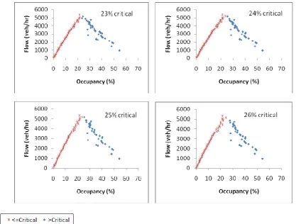
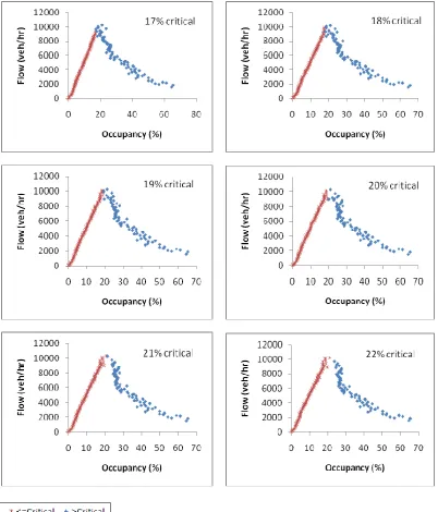
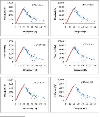
Before applying the average occupancy approach for each corresponding flow, the data is filtered to

remove the transition cases from congested to normal traffic situations. Figures 3, 4, 5 and 6 show the

possible shapes for flow-occupancy relationships for different trials of critical occupancy values using the

approach of average occupancy at each specific flow for the M56 J2, M6 J23, M6 J20 and M60 J2,

respectively. For the M56 J2, Figure 3 shows that the critical occupancy value lies between 25 and 26%.

Lower values are not considered because these lower values give flows for congested regime that are

equal or higher to those in a normal regime.

In the same way, and based on Figures 4-6, values of 23%, 22% and 20-21% are suggested for the M6

J23, M6 J20 and M60 J2, respectively:

(28)

[image:28.595.67.484.153.469.2]

(29)

[image:29.595.69.471.155.625.2]

(30)

[image:30.595.69.473.155.625.2]

(31)

[image:31.595.73.472.157.643.2]

(32)

Figure 7 gives examples about critical occupancy values based on the time series inspection approach. It

should be noted that only congested situations caused by merge traffic are considered (i.e. congested

situations due to further downstream bottlenecks are not considered). While the results obtained from the

first method (average occupancy) gave limited variation in critical occupancy between sites, the variation is

more announced using the time series inspection method. This variation is also described in the work by

Hall et al. (1986).

Figure (7) Critical occupancy values using time series inspection method

Table 1 compares the critical occupancy values obtained from the average occupancy approach with such

critical values that are currently in use to trigger the ramp metering devices on the selected motorway

sites. The value that is used to trigger the ramp metering in M56 J2 was not given due to a lack of data.

The table shows that for the M6 J23 and M6 J20 sites, the values which are currently used to operate the

[image:32.595.67.461.275.615.2]

(33)

cause delays in the operation of the RM after the traffic congestion has started and that ultimately causes

reduction in motorway throughput. For the M60 J2, the value used is much close to the estimated value.

Table 1 Estimated and Values in use for critical occupancy

Site M6 J23 M6 J20 M60 J2

Estimated critical occupancy (%)

23 22 20-21

Value in use in RM (%) 28 25.5 19

5. Summary

This paper focuses on the estimation of critical occupancy using data taken from loop detectors. The data

from four motorways junctions which are served by ramp metering devices in the UK are used. These

motorways are M56 J2, M60 J2, M6 J23 and M6 J20. Two methods are used to find the critical

occupancy. The first method is by finding the average occupancy for each corresponding flow. The

second method is to follow-up the transitions from normal to congested situations. It is found that the

variation between the results between the selected sites is more pronounced using the second method.

The results are compared with corresponding values as adopted by the Highways Agency for these sites

to operate the ramp metering. As a part of M60 J2, the results show that the values which are currently

used to operate the ramp metering devices in these sites are higher than those obtained from analysing the

data. This will cause delays in the operation of the RM until the starting of traffic congestion which

ultimately causes reduction in motorway capacity.

6. References

Hall, F. L., Allen, B. L. and Gunter, M. A., (1986). Epirical analyses of freeway flow-density

relatioships. Transportation Research A, Vol. 20A, No. 3 p.p. 197-210.

Masher D.P., Ross D.W., Wong P.J., Tuan P.L., Zeidler H.M., and Petracek S., (1975), Guidelines for

Design and Operation of Ramp Control Systems", Stanford Research Institute, Menid Park, CA.

(34)

Papageorgiou, M., Haj-Salem, H. and Blosseville, J-M. (1991). "ALINEA: a local feedback control law

for on-ramp metering." Transportation Research Record, Volume (1320), p.p. 58-64.

Papageorgiou, M., Haj-Salem, and F. Middleham, (1997), ALINEA local ramp metering: Summary of

field results. In Transportation Research Record 1603, TRB, National Research Council, Washington

D.C., 1997, pp. 90-98.

Sarintorn, W. (2007) Development and comparative evaluation of ramp metering algorithms using

microscopic traffic simulation. Journal of Transportation, Volume (7), Issue 5, p.p. 51-62.

Smaragdis, E., Papageorgiou, M. and Kosmatopoulos, E. (2004) A flow-maximizing adaptive local ramp

metering strategy, Transportation Research Part B: Methodological, Volume (38), Issue 3, p.p. 251-270

Zhang, L. and Levinson, D. (2010) Ramp metering and freeway bottleneck capacity Transportation

(35)

The Effects of Residential Location on Total Person Trip Rates:

An Empirical Study

Firas Asad,School of Computing, Science and Engineering, University of Salford

1. Introduction

Developing a robust trip generation model, for predicting the number of vehicular/person trips generated

by a residential development, is still a vital task for both transportation planners and engineers. There are

two key reasons for this; one of them is because trip generation is the first model in the travel forecasting

process for the vast majority of orthodox urban transportation modelling systems (UTMSs). The second

reason is because local planning agencies need the predicted number of trips that are likely to be

generated from a proposed development to quantify the anticipated impacts of such development on the

transport system infrastructure and performance.

Consequently, many researchers have been studying the factors that possibly affect the total number of

the generated trips (trip ends). Site location as one of the residential land use descriptive characteristics, is

one of the relevant factors to be studied. The objective of this paper is to investigate whether the location

of a residential site affects its trip-making pattern and hence its traffic impacts as an attempt to attach a

spatial dimension of study to the land use-trip generation relationship.

The Trip Rate Information Computer System (Trics-ver.2009a), being one of the UK and Ireland’s

industry standard trip generation database, is interrogated in this study. It is used to derive the likely mean

person and vehicle trip ends for residential sites with six different location types and for, where possible,

six modes of travel. The statistical methodology ANOVA (Analysis of Variance) using SPSS (ver.17,

2008) software is employed to examine whether there are any statistically significant differences among

the trip rates means of Trics main location groups for each travel mode separately.

2. Trics Database

Trics was founded and is owned by the Trics Consortium, which consists of 6 county councils (West

Sussex, East Sussex, Surrey, Kent, Dorset, and Hampshire). It is the national standard for trip generation

analysis, containing about 6,000 directional transport surveys at more than 100 types of land uses in the

(36)

At the start of the trip rate calculation process, after selecting the proper land use category and

subcategory, Trics asks the user, through a number of windows with user-friendly interface, to provide

the system with a series of initial, main, secondary, and optional parameters. By specifying these

parameters users can create their representative sample of sites. In the initial parameters window, the user

is required to choose between vehicle-based and modal trip rate calculation options. In the

multi-modal option, trip rates and/or the total number of arrival, departure and total trips (both direction) can be

computed for travel modes other than total vehicles like, for instance, pedestrians, cyclists, PTUs, and

total people.

In the next stage, the main parameter window, the primary trip rate parameter like number of dwellings,

total bedrooms or site area should be firstly chosen followed by the desired week days and finally the

main and secondary site location types. After that, in the secondary stage, desired sites and survey days

should be determined. Finally, further fine-tuning for the sites may be done by optional parameters

including population, car ownership and access to a travel plan.

Trics, in line with the planning policy statement 6 (PPS6, 2005), assigns main and, where applicable,

sub-location definitions as a descriptive characteristic for each development site. The main location

categories are basically as a proxy measure of how far is the site from the central core area of the

town/city. The availability of public amenities is also a major determinant in location definition. In Trics

2009(a), being interrogated in this study, there are six main location categories; Town centre TC, Edge of

town centre ETC, Neighbourhood centre NC (Local centre), Suburban area SA (Out of centre), Edge of

town ET, and Free standing FS (Out of town). For more information and definitions, interested readers

are referred to the Trics 2009(a) online help. Taking into account the basic requirement for a statistically

adequate sample size, only the main six location types are considered in this analysis. On the other hand,

the total vehicle counts in addition to five of the multi-modal trip rate counts are included in the statistical

analysis. These five multi-modal counts are: total people, pedestrians, vehicle occupancy, PTUs, and

motor cars.

There are 13 residential land use subcategories (sub land uses) in Trics (2009a); only seven of them were

chosen to be interrogated in this study. These seven are; Houses Privately Owned (HPO), Houses for Rent

(HFR), Flats Privately Owned (FPO), Flats for Rent (FFR), Mixed Private Housing (MPH), Mixed

(37)

A full definition of these residential developments is available in the Trics 2009 Online Help File. Other

subcategories were excluded either for lack of an adequate number of sites (in this study a threshold of

more than 3 sites is adopted), or because of the inconsistency in the trip generation calculation parameter.

For all the seven selected subcategories, the number of dwelling units is adopted as a unit of analysis in

calculating the vehicle and person weekday trip rates. The Guidance on Transport Assessment (2007)

reports that for residential developments the peak periods predominantly occur on weekdays, hence

surveys selected in this study were based on a 12hr. (7.00-19.00) weekday analysis period.

In line with Trics recommendations (Trics Basic Tutorial, 2005), only the most recent surveys were

chosen to avoid any possible bias towards the multiple survey sites. Furthermore, in order to keep the

subcategory datasets as eligible as possible for statistical analysis, no further filtering has been applied by

Trics optional parameters. In Table 1, each cell shows the available number of multi-modal counts sites in

Trics 2009(a) for each specific residential land use and location type. Unfortunately, this pilot survey

evidently reveals that most of these cells are ineligible for statistical analysis according to this study

threshold (more than 3 sites).

Table 1: Trics 2009(a) multi-modal counts sites cross classified by both residential land use and location

types

Land use / Location Types Town

centre

Edge of

town

centre

Neighbour

hood

centre

Suburban

area

Edge of

town Free Standing

A. Houses privately owned 0* 6 2* 30 28 0*

B. Houses for rent 0* 2* 0* 5 1* 0*

C. Flats privately owned 3* 10 0* 10 0* 0*

D. Flats for rent 0* 7 0* 9 4 0*

K. Mixed private housing 1* 2* 1* 13 3* 1*

L. Mixed non private housing 0* 2* 0* 1 0* 0*

M. Mixed private/non private

housing

0* 0* 0* 8 6 0*

*

Not sufficient for statistical analysis.

To avoid this, a proposed regrouping of the seven Trics 2009(a) residential subcategories, produced by

Asad and Henson (2010) has been adopted. Based on a statistically grounded methodology and the

category analysis method concepts, Asad and Henson (2010) showed that these seven residential

(38)

As a consequence, a new grouping consisting of two main housing subcategories has been produced,

namely; Houses-like travel behaviour (HLTB) and Flats-like travel behaviour (FLTB). The first housing

subcategory, HLTB, contains four of the seven original Trics residential subcategories; Houses-privately

owned, Houses for rent, Mixed non-private housing, and Mixed private/non-private housing. In contrast,

Flats-like TB housing group contains the remaining three; Flats privately owned, Flats for rent, and

Mixed private housing.

3. Site Location

The Trics good practice guide (2009, p.4) pointed out that site location type is one of the vital data fields

when seeking site selection compatibility. Six main location categories are listed in Trics 2009a, and all

of them, where possible, are considered here. The guide further stated that development sites located in a

town centre will experience a modal split different from another site in rural areas when there is a

considerable variation in the acceptable level of local public transport accessibility.

Many researchers have highlighted the issue of how the travel behaviour of a specific land use may be

affected by its location type. Hurst (1970) stated that land use location, relative to the central business

district (CBD/Non CBD), is a principal variable in the functional relationship between a non-residential

land use and urban travel volume. Baumgaertner (1985) for example, found that trip generation rates for

movie theatre in urban areas are quite different from those in suburbs. Three modes of travel were

included in the study; passenger vehicles, pedestrian and rail/bus.

Szplett and Kieck (1995), depending on household travel surveys from two cities, demonstrated that

household location with respect to the city centre has a clear impact on the number of generated vehicle

trips. In addition, they revealed that downtown residents generate vehicle trips more than those living in

suburban environments. Boarnet, et al. (2003) in their statistical research found out that non-work trip

frequency, in the developed ordered probit model, significantly depends on a set of sociodemographic and

land use variables. Residence location relative to the CBD was found to be one of them. Rhee (2003)

emphasised that in constructing the cross classification table in the category analysis method, households

are categorised according to a set of attributes such that trip production characteristics within each

category are similar. Household location is one of these attributes employed for stratification.

Three recent relevant studies have been found during reviewing previous studies. O’Cinneide and Grealy

(2008) studied the likely primary factors that would quantify the traffic volume generated from residential

(39)

compared with Trics equivalent rates. It was revealed that development location mainly influences the

morning peak traffic generation frequency, type of occupant, and car ownership level. Three location

types were included; inner city, suburbs, and rural areas. The study claimed that car trip rates for inner

city/town development are, in general, lower than those rates in suburbs or rural areas. However, no

statistical evidence was employed to show how significant is the location effect on the residential traffic

generation.

Maclaine (2007) based on Trics 2007(a) site characteristics and count data and the correlation statistical

technique results, showed that no significant correlation was found between the multi-modal count data

and the Trics 2007 optional parameter; location. Therefore, the study stressed that refining the sample

according to the main location parameter is not recommended. It is worthwhile noting that the Pearson

correlation coefficient (r) was used as a parametric test, although no statistical evidence was presented to

show both the normality of the correlated variables and their variance homogeneity. Furthermore, the

Pearson correlation coefficient was computed for two variables; one is continuous (trip rate) while the

other is categorical (location). Nevertheless, the study failed to submit an illustrative example to

demonstrate how that was done.

Broadstock (2008, 2009), using Trics 2004(b) as the main database, researched the possible effect of land

zone placement, in line with spatial planning policy, on passenger car trip making behaviour in residential

areas. Depending on a semi-parametric regression technique and bootstrap algorithm, the study concluded

that geographical features such as land zone placement marginally determine residential car trip

generation rates. Broadstock (2009, p.19) claimed that “there are no individually significant land zone

variables, yet they represent a statistically relevant feature of the final preferred model”. Hence, no

powerful proof has been produced on the proposed functional relationship between land zone placement

and travel behaviour.

Two key points should be highlighted in both of Broadstock’s studies; the first is the data constraint in

Trics during the selected period of study (1987-2002) (Broadstock, 2008, p.145). The second is the use of

a semi-parametric technique instead of a robust parametric one due to the issues of small sample size and

variance heterogeneity (Broadstock, 2008, p.2). Finally, the study has failed to properly distinguish

between the 14 Trics 2004(a) residential sub land uses when analyzing land zone impacts on travel

behaviour. In particular, the study considered all the 14 sub land uses as one single residential group

(40)

4. Study Methodology

For obvious statistical reasons it is highly recommended when studying the probable effect of a specific

factor (independent) on the behaviour of a certain variable (dependent) to exclude the possible effects of

other factors that may influence the dependent variable behaviour. For applying this scenario here, it is

supposed to isolate the impacts of other socio-economic and development type factors when studying the

effects of housing development location type on its trip making patterns.

However, the Trics 2009(a) database in its current depth and breadth of records makes it statistically

impractical to filter data like that. According to the vast majority of trip generation literature, the type of

development has a significant effect on the trips generated, consequently, only this factor is considered in

this study. Furthermore, the scientifically grounded new housing groupings suggested by Asad and

Henson (2010) for Trics 2009(a) residential land uses is adopted; Houses-like TB and Flats-like TB.

It is useful to recall that the effect of the six housing location types on the number of trips generated was

examined separately for each of the two new housing groupings. As mentioned previously, six types of

travel modes have been adopted; total vehicles, motor cars, PTUs, pedestrian, vehicle occupancy, and

total people. Total vehicle counts were extracted from the vehicle trip rate option in the Trics 2009(a) trip

rate calculation initial parameter window. In contrast, the other travel modes count data were calculated

using the multi-modal trip rate option. For each mode of travel mentioned above, the statistical procedure

one-way ANOVA has been employed to test whether there is a significant difference between the trip rate

means (dependent variable) of the six selected location types. This is done for each housing group

separately.

Using SPSS (ver.17) the Least Significant Difference (LSD) method is employed to investigate the

potential differences between sample group means (with a null hypothesis Ho : there is no significant

difference) at 5% level of significance (LOS). Moreover, using the ANOVA post – hoc analysis

technique, multiple comparisons could be performed to discover which specific group mean (mean of a

specific trip rate location category) may significantly differ from others and by how much (George and

Mallery, 2009).

Being one of the robust parametric statistical tests, ANOVA depends on restrictive main conditions, like

normality and variance homogeneity. The data in the groups being tested should be independent and

drawn from a population that is normally distributed and these groups should have variances not

substantially different from each other (Keller, 2005). Based on Shapiro-Wilk (S-W) and

Kolmogorov-Smirnov (K-S) normality tests embedded in SPSS, it has been found that some of location groups have

(41)

This problem has been solved by applying a logarithmic transformation of type (y = ln(x)) for these

groups’ observations. This mathematical solution has been suggested and supported by many researchers

(for example see Bland and Altman (1996) and Osborne (2002)). On the other hand, Levene’s test is used

to examine whether the between-groups variances are substantially heterogeneous (Heteroskedasticity).

Hayter (2007) emphasised that both of these conditions could be considered satisfied unless they have

been violated remarkably, i.e., either the data are obviously not normally distributed or there is a

significant difference between the variances of the levels (location categories) of the factor (trip rate)

being analysed.

5. Data Analysis Results and Discussion

The limited count data for modes of travel at some location categories is the reason behind excluding

some statistics from the analysis. For instance, there is no data for HLTB housing in town centres,

whereas, both neighbourhood centre and free standing locations were mostly excluded for the shortage of

a statistically efficient sample size. The trip rate figures are the total (arrivals and departures) 12hr.

(7:00-19:00) expected trips per each dwelling unit. In the following subsections the analysis results of the effect

of site location on trip making pattern will be shown and discussed for each type of traffic counts. The

level of significance (LOS) is 0.05 (5%) for all the inferential statistical analysis unless stated otherwise.

a. Total vehicles

This count includes all vehicles entering and exiting a site at any access point excluding cyclists. For

HLTB housing, Table 2 shows the SPSS normality tests output for the total vehicles trip rate (VehTR)

dependent variable. It is clear that approximately all the location groups have data that are normally

distributed at 5% LOS according to Shapiro-Wilk test. Although, ET location group are significantly

different from normality using S-W test, however, it does not show significant deviation from normality

at 0.10 LOS using K-S test (Sig.= 0.02). As a result, no more concerns were devoted to the normality

assumption of the ANOVA model and therefore a logarithmic transformation was not adopted in this

(42)

Table 2. Tests of Normality results for HLTB housing.

Location Type

Sig. (P-value)

Kolmogorov-Smirnova

Shapiro-Wilk

VehTR Edge of Town Centre ETC .103 .166

2Neighbourhood Centre NC (PPS Local Centre)

.200* .444

Suburban Area ( PPS Out of Centre) .200* .633

Edge of Town .022 .002

Free Standing (PPS Out of Town) .299

a. Lilliefors Significance Correction

Table 3 shows the output results of the Levene’s test for the homogeneity of variances

(Homoskedasticity). The statistics do not prove any distinct variation (P-value = 0.237).

Table 3. Test of Homogeneity of Variances

Levene Statistic df1 df2 Sig.(P-value)

1.394 4 249 .237

The results of the ANOVA model are found to be significant with P-value (Sig.) equal to 0.008. This

means there is at least one location group with trip rate mean significantly deviate from others. Post-hoc

tests using the LSD method may now be carried out. Table 4 presents the HLTB housing group multiple

comparisons. The statistical analysis results (see table 4) reveal that edge of town ET trip rate is

significantly larger than vehicle trip rate in both edge of town centre ETC and neighbourhood centre NC

[image:42.595.64.480.176.404.2]

(43)

[image:43.595.65.494.178.544.2]

Table 4. Multiple Comparisons results using LSD method.

(I) LocCode (J) LocCode Mean Difference (I-J) Std. Error

Sig.(P-value)

Edge of Town Centre Neighbourhood Centre -.129508 .487426 .791

Suburban Area -.675883 .445967 .131

Edge of Town -1.055186* .432593 .015

Free Standing -.582964 .870230 .504

Neighbourhood Centre Edge of Town Centre .129508 .487426 .791

Suburban Area -.546375 .316059 .085

Edge of Town -.925678* .296890 .002

Free Standing -.453456 .811361 .577

Suburban Area Edge of Town Centre .675883 .445967 .131

Neighbourhood Centre .546375 .316059 .085

Edge of Town -.379303 .222365 .089

Free Standing .092919 .787152 .906

Edge of Town Edge of Town Centre 1.055186* .432593 .015

Neighbourhood Centre .925678* .296890 .002

Suburban Area .379303 .222365 .089

Free Standing .472222 .779653 .545

Free Standing Edge of Town Centre .582964 .870230 .504

Neighbourhood Centre .453456 .811361 .577

Suburban Area -.092919 .787152 .906

Edge of Town -.472222 .779653 .545

*. The mean difference is significant at the 0.05 level.

Table 4 presents the full SPSS output for this case. However, to avoid excessive length, SPSS results for

the remaining comparisons will be limited to summary results rather than full tabulations.

For FLTB, Similarly, ANOVA primary conditions (normality and homoskedasticity) should be at first

satisfied before performing the multiple comparisons. Natural log transformation was done for data since

there was significant deviation from the normality for some of them. The post-hoc tests results show that

town centre TC trip rate is substantially lower than other locations’ rates. Furthermore, no significant

distinctions in trip rates are noticed between edge of town ET, suburban area SA, and neighbourhood

centre NC locations. However, it seems that people in ET locations use vehicles more than those living

near TC. Fig. 1 shows that, in general, there is an increase in the total generated vehicles with the increase

Conference proceedings 2010

Conference proceedings 2010

SPARC,

Title

Conference proceedings 2010

Authors

SPARC,

Type

Conference or Workshop Item

URL

This version is available at: http://usir.salford.ac.uk/16822/

Published Date

2010

USIR is a digital collection of the research output of the University of Salford. Where copyright

permits, full text material held in the repository is made freely available online and can be read,

downloaded and copied for non­commercial private study or research purposes. Please check the

manuscript for any further copyright restrictions.

Proceedings of the

Salford Postgraduate Annual

Research Conference

(SPARC)

2010

Preface

Contents

Evaluation of Car-following Models Using Field Data

Estimation of critical occupancy values for UK motorways from traffic loop detectors

The Effects of Residential Location on Total Person Trip Rates:

An Empirical Study

downloaded and copied for noncommercial private study or research purposes. Please check the