Munich Personal RePEc Archive
Structural estimation of the
New-Keynesian Model: a formal test of
backward- and forward-looking
expectations
Jang, Tae-Seok
University of Kiel
25 June 2012
Structural estimation of the New-Keynesian model:
a formal test of backward- and forward-looking expectations
Tae-Seok Jang
∗1
Department of Economics, University of Kiel (CAU), Germany
June 25, 2012
Abstract
This paper attempts to uncover the empirical relationship between the price-setting/consumer
be-havior and the sources of persistence in inflation and output. First, a small-scale New-Keynesian
model (NKM) is examined using the method of moment and maximum likelihood estimators with
US data from 1960 to 2007. Then a formal test compares the fit of two competing specifications in
the New-Keynesian Phillips Curve (NKPC) and the IS equation; i.e., forward- or backward-looking
expectations. Accordingly, the inclusion of a lagged term in the NKPC and the IS equation improves
the fit of the model while offsetting the influence of inherited and extrinsic persistence; it is shown
that intrinsic persistence plays a major role in approximating the inflation and output dynamics for
the Great Inflation period. However, the null hypothesis cannot be rejected at the 5% level for the
Great Moderationperiod; i.e. the NKM of purely forward-looking behavior and its hybrid variant are
equivalent. Monte Carlo experiments illustrate the validity of the chosen moment conditions and the
finite sample properties of classical estimation methods. Finally, the empirical performance of model
selection methods is investigated using the Akaike’s and the Bayesian information criterion.
JEL Classification: C12, C32, E12, G12
Keywords: formal test, foward- and backward-looking expectations, information criterion,
intrinsic persistence, maximum likelihood, method of moment, New-Keynesian model
∗This paper was presented at the seminars in CAU and the 10th AnnualAdvances in EconometricsConference at SMU.
I have benefited from discussions with Reiner Franke, Ivan Jeliazkov, Vadim Marmer, Fabio Milani and Stephen Sacht.
I also express my gratitude to all the participants for their active involvement in the conference. The support from the
German Academic Exchange Service (DAAD) and the M¨oller fund from CAU is greatly acknowledged. Address of author:
1
Introduction
In the New-Keynesian model (NKM), some extensions such as the habit formation and indexing behavior have gained popularity for the ability to fit the macro data well; see Christiano et al. (2005), Smets and Wouters (2003, 2005, 2007) and Rabanal and Rubio-Ramarez (2005). For instance, the forward-looking behavior of price indexation has been challenged by macroeconomists over the last decade, because a hybrid variant of the model with the backward looking expectations provides a good approximation of inflation dynamics; see also Gali and Gertler (1999), Fuhrer (1997), Rudd and Whelan (2005, 2006), and many others. In the same way, inertial behavior in the dynamics of the output gap can be better explained by the presence of the habit formation in consumption rule; e.g. see Fuhrer (2000). Accordingly, the lagged dynamics in the NKM influence the transmission of shocks to the economy; the backward-looking behavior in the price-setting/consumption rules increases the degree of endogenous inflation/output persistence. This also implies that a good approximation of the NKM to the data (e.g. the persistence of aggregate macro variables) can provide a potential explanation for the monetary transmission channel to inflation and output; see Amato and Laubach (2003, 2004).
In a small-scale hybrid NKM, however, inflation and output depend on its expected future and lagged values, which induce a non-linear mapping between structural parameters and the objective function during estimation. Because of this, the structural system cannot avoid identification problems in the model; in other words, the minimization problem in extreme estimators often does not ensure a unique solution asymptotically; e.g. see Canova and Sala (2009). The purpose of this paper is to show to what extent classical estimation methods can cope with strucutural parameter estimates and how they can be used to evaluate the model’s empirical performance. In particular, we focus on a system estimator which is based on an analytical solution of the model in estimation.1
More generally, to examine the significant influence of the lagged inflation and output on the structural dynamics, we apply the formal test of Hnatkovska, Marmer and Tang (2012) [HMT henceforth]. According to HMT, the Vuong-typeχ2test accomodates the adequacy of a broad class of the goodness-of-fit measures,
which allow for model misspecifications; see also Linhart and Zucchini (1986) for model selection. Hence, the test statistic used herein can evaluate the discrepancy between the model-generated and empirical moments, which is associated with the goodness-of-fit of the model. With regard to the hypothesis testing, for example, the likelihood ratio test has been extensively used for non-nested hypotheses due to Vuong (1989). Rivers and Vuong (2002) generalized normal tests for model selection problems to the application involving a broad class of estimation methods. Their procedure extends to somewhat complex model selection situations where one or both models may be misspecified and the models may or may not be nested; see Golden (2000, 2003).
The advantage of the formal test of HMT is that the model’s empirical performance can be flexibly evaluated according to the chosen moment conditions. The flexibilty is associated with the transparency to
1
Alternatively, the common and simple strategy to provide a quantitative assement of inflation and output is to use a
reduced form (or single equation) estimation, calibration or simulation based inference; see also Gregory and Smith (1991),
the fit of the model when the moment conditions are directly binding for parameter estimation. Indeed, the limited information approach has been widely used to estimate parameters of the DSGE models starting from Rotemberg and Woodford (1997). For instance, one common approach to this problem is to use impulse responses that are most informative about the DSGE models; Dridi et al. (2007) and Hall et al. (2011) discussed the choice of binding functions and information criteria for the selection of the valid response. Especially, when the model misspecifications and complex structural system do not allow for efficient estimation, the adequacy of the model in fitting the data can be judged by using binding functions; see Gourieroux and Monfort (1995). To provide parameter estimates using the limited information approach without auxiliary model, Franke et al. (2011) examined a small-scale DSGE model with analytical second moments of the sample auto- and cross-covariances up to lag 8 (two years) for estimation as well as model selection. While their empirical results are contrasted with the ones estimated by a Bayesian approach, however, the set of valid moment conditions is not tested.
In this paper, we discuss the efficiency of the method of moments (MM) estimation and examine the validity of moment conditions in comparison with the maximum likelihood (ML) approach. To see this, first, we study the relationship between interest rate, inflation and the output gap for US data, and provide a thorough analysis on empirical performance of the model and its connection to the expectation formation process: backward- and forward-looking behavior. From the ML and MM parameter estimates of the NKM, we pinpoint an empirical link between the hybrid model structure and the persistence in inflation and output. Next, the emprical performances of the NKM of purely forward and its hybrid variant are evaluated according to the model selection criterion. Accordingly, the inclusion of a lagged term in the New-Keynsian Phillips Curve (NKPC) and the IS equation improves the fit of the model while offsetting the influence of inherited and extrinsic persistence; it is shown that intrinsic persistence plays a major role in approximating the inflation and output dynamics for theGreat Inflation period. However, the null hypothesis cannot be rejected at the 5% level for theGreat Moderation period; i.e. the NKM of purely forward-looking behavior and its hybrid variant are equivalent. Finally, we also carry out a Monte Carlo (MC) study to examine the statistical efficiency of the estimation methods.
2
Expectation formation in a DSGE model
In this section, we present the standard New-Keynesian model featuring aggregate supply (AS), aggregate demand (IS), and monetary policy equations.2 We focus on the model specifications for the expectation
formation in the NKPC and the IS equation.
2.1
The New-Keynesian three-equations model
Microfoundations of supply- and demand-side economy have been established as the key components of a New-Keynesian model framework; e.g. the behavior of optimizing economic agents. The monetary policy behavior is described by the Taylor rule where the lagged interest rate reflects gradual adjustment of central banks. Thus the model is applicable to the dynamic analysis of economic changes. More generally, we attempt to examine the extent to which the gaps of interest rate, inflation and the output influence each other and affect the economy (bπt:=πt−πt∗, brt:=rt−rt∗). The trend components of the quarterly
data are estimated by using the Hodrick-Prescott filter with the smoothing parameter ofλ=1600.3
b
πt = β
1 +αβ Etπbt+1 + α
1 +αβ πbt−1 + κ xt + νπ,t
xt = 1
1 +χ Etxt+1 + χ
1 +χ xt−1 − τ (brt−Et bπt+1) + νx,t (1) b
rt = φrrbt−1 + (1−φr) (φππbt+φxxt) + εr,t
νπ,t = ρπνπ,t−1 + επ,t (for indexing behavior) (2) νx,t = ρxνx,t−1 + εx,t (for consumption behavior)
where the variablextdenotes the output gap,πbtthe inflation gap andbrtthe interest rate gap. The discount
factor and the slope coefficient of the Phillips curve are denoted by the parametersβ andκrespectively. The parametersα and χ measure the degree of price indexation in the NKPC (0 ≤α ≤ 1) and habit formation of the household (0≤χ≤1) whileτ relates to the intertemporal elasticity of substitution of consumption (τ ≥0). In the Taylor rule,φrdetermines the degree of interest rate smoothing (0≤φr≤1).
The other parametersφx andφπ are the policy coefficients that measure the central bank’s reactions to
contemporaneous output and inflation (φx, φπ ≥0).
The shocksεz,tare normally distributed with standard deviationσz (i.i.d. withz=π, x, r). Sinceνπ,t
andνx,tare autoregressive processes, the persistences of the cost-push and the supply shocks are captured
2
Smets and Wouters (2003, 2007) developed a medium-scale version of the NKM and estimated structural parameters
and idiosyncratic shocks with the Bayesian techinques. In our study we focus on a small-scale general equilibrium model
where we attempt to investigate the role of optimizing behavior in inflation and the output gap dynamics.
3
Note here that we use the gaps instead of the levels for interest rate and inflation. Indeed, many empirical studies
provide evidence for a time-varying trend in inflation and the natural rate of interest; see Castelnuovo (2010), Cogley and
Sbordone (2008), Cogley et al. (2010) and many other studies. Further, the second moments are chosen to match the data
when we estimate the model parameters. As a result, if we would use the non-stationary data without making assumptions
by the parametersρπ andρx, respectively (0≤ρπ, ρx≤1). In estimation, we do not take them together,
but treat them as being an independent case in order to directly disentangle the sources of inflation and the output gap persistence in the model.4
We denote yt by the state vector of three variables: yt= (bπt, xt, rbt)′. For the sake of simplicity, we
present the above structural equations into the following canonical form:
AEtyt+1 + Byt + Cyt−1 + νt = 0 (3)
νt = N νt−1 + εt, εt∼N(0,Σε)
With regard to the solution of the system, we begin with matrices Ω and Φ in the recursive equation of the reduced form. First, we use the method of undetermined coefficients to obtain the unique solution of the system under determinacy (i.e.,φπ≥1). Second, we apply the brute force iteration method of Binder
and Pesaran (1995) to numerically evaluate the matrix Ω; see appendix B for some intermediate steps.
yt = Ωyt−1 + Φνt (4)
νt = N νt−1 + εt
From the matrices Ω and Φ, it follows that the contemporaneous and lagged autocovariance process of the model can be computed recursively using theYule-Walker equations; see chapter 2 of L¨utkepohl (2005). On the whole, we only need to adjust the notation by changing the dating of the shocks and rewrite Equation (4) as
yt
νt+1
=
Ω Φ
0 N yt−1
νt +
0
I
εt+1 (5)
With zt = (yt′, νt′+1)′, D = (0 I)′, ut =Dεt+1, and A1 the 2n×2n matrix on the righthand side
associated with the vector (y′
t−1, νt′)′ =zt−1, Equation (5) can be more compactly written as
zt = A1zt−1 + ut, ut∼N(0,Σu), Σu=DΣεD′ (6)
where the matrixA1and the covariance matrix Σuare functions of the parameter vectorθ. The estimation
methodologies will be discussed later.
4
The present study does not consider the presence of serially correlated shocks in the realizations of interest rate. It is
2.2
Sources of persistence: backward- and forward-looking behavior
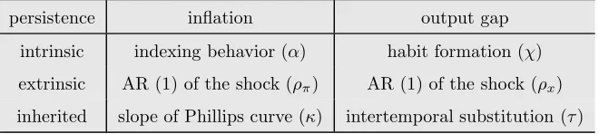
[image:7.595.139.469.244.318.2]In the study of the model comparison, we put our focus on two polar cases of expectations. For example, when the price indexation parameterα is set to zero, it is assumed in the model that expectations are purely forward-looking. In this case, inflation persistence is exclusively driven by the exogenous shock process and inherited persistence from the output gap (see Table 1). But allowing it to be a free parameter, we assume that agents in the market form the backward-looking expectations. As a result, the NKPC is affected by both expected future and lagged inflation.
Table 1: Sources of persistence in the NKPC and the IS equation persistence inflation output gap
intrinsic indexing behavior (α) habit formation (χ) extrinsic AR (1) of the shock (ρπ) AR (1) of the shock (ρx)
inherited slope of Phillips curve (κ) intertemporal substitution (τ)
In the same vein, Table 1 shows that we can test the backward and forward-looking behavior in the IS equation. As long as each household chooses consumption optimally (i.e., without habit formation,
χ = 0), the persistence of the output gap is only driven by the exogenous shock and the inherited persistence implied by the Euler condition for the optimality intertemporal allocation of consumption. On the contrary, if habit formation is present in the consumption rule (i.e.,χis now a free parameter), then the output gap dynamics are endogeneously sustained by the optimizing behavior. As a result, the NKPC also depends on the lagged and expected future output gap.
3
Estimation methodologies and model selection
This section studies the structural estimation of the NKM when an analytical solution of the model is known. We also present the way in which a formal test can be used to evaluate the competing models.
3.1
Method of moment and model comparison: HMT (2012)
From the law of motion in Equation (6), it follows that the second moments of zt can be analytically
computed. Thus the contemporaneous and lagged autocovariances of the first-order vector-autoregressive (VAR (1)) are given by:
Γ(h) := E(ztzt′−h)∈RK
×K, K= 2n, h= 0,1,2,
· · · (7)
Their computation proceeds in two steps. First, Γ(0) is obtained from the equation Γ(0) =A1Γ(0)A′1+
Σu, which yields
vecΓ(0) = (IK2−A1⊗A1)−1vecΣu (8)
where the symbol ’⊗’ denotes the Kronecker product and invertibility is guaranteed, becauseA1is clearly
a stable matrix; i.e. φπ ≥1. Subsequently the Yule-Walker equations are employed, from which we can
recursively obtain the lagged autocovariances as
Γ(h) = A1Γ(h−1) (9)
This formula relates to a vector autoregressive process of the model. From Equation (9), it follows that the model-generated second moments can be used to match the empirical counterparts in the MM estimation. In order to compare the empirical performance of two models (A and B), first we must estimate the model parameters by minimizing a weighted objective function (chosen goodness-of-fit measures):
JI(θ)≡ min
θI∈Θ
W1/2(
b
mT−mI(θI)) 2
, I=A, B (10)
where mI is a vector of moments and mb is a consistent and asymptotically normal estimator of true
momentsm0. The norm of the matrixX is defined as||X||=
p
tr(X′X), where tr denotes trace.
the output gap (xt), and the inflation rate gap (πbt); see also appendix A. As for the alternative moment
conditions, we make use of the auto- and cross-covariances up to lag 4 (42 moments). The results of empirical findings and their robustness will be discussed later. Indeed, the second moments are applicable to the evaluation of the NKM’s empirical performance and its comparison to the other specification.
In order to construct the objective function, we must estimate the weight matrixW using the Newey-West estimator (Newey and Newey-West (1987))5:
b
ΩN W =ΓbT(0) +
5
X
k=1
b
ΓT(k) +ΓbT(k)′
(11)
where bΓT(j) is T1 PTt=j+1(mt−m¯)(mt−m¯)′ and k is the number of lags.6 Note here that we use the
diagonal components of the weight matrix and compute the inverse of ΩbN W; here we impose the zero
off-diagonal element restriction on the matrixΩbN W, because the elements of the weight matrix and the
moments are highly correlated in a small sample size (see Altonji and Segal (1996)).
Under standard regularity conditions, the asymptotic distribution of the parameter estimates is given by:
√
T(θbT −θ0)∼N(0,Λ) (12)
where we can numerically compute the covariance matrix Λ using the first derivative of the moments at the optimum (Λ = [(DW D′)−1]D′WΩW D[(DW D′)−1]′).7 Note here that D is a gradient vector of
moment functions evaluated at the estimated points:
b DT =
∂m(θ;XT) ∂θ
θ=bθT
(13)
Next, we consider hypotheses comparing the goodness-of-fit of the competing models. The null hy-pothesisH0 is that two non-nested models fit the data equally:
H0:
W1/2(
b
mT −mA(θA))
−W1/2(
b
mT −mB(θB))
= 0 (14)
5
If large lags are included in the moments to be matched, the rows in the weight matrix are correlated to some extent.
To avoid the dependence of the moments, we employ diagonal components of the Newey-West variance-covariance matrix in
computing the weight matrix.
6
The lag order is chosen following a simple rule of thumb for sample size (∼T1/4
). For the GI and GM data, we have 78
and 99 quarterly observations respectively. Therforekis set to 5.
7
If the weight matrix is chosen optimally (cW= Ω−1
), Λ becomes (DW D′)−1
; see chapter 1 of Anatolyev and Gospodinov
(2011) among others. However, in our study, the estimated confidence bands become wider, because the weighting scheme
The first alternative hypothesis is that modelA performs better than modelB when
H1:
W1/2(mbT −mA(θA))
−W1/2(mbT −mB(θB))
<0 (15)
The second alternative hypothesis is that modelB performs better than modelAwhen
H2:
W1/2(mbT −mA(θA))
−W1/2(mbT −mB(θB))
>0 (16)
To carry out the model comparison, we define the quasi-likelihood-ratio (QLR) statistic as
[
QLR =JB(θbB)−JA(θbA) (17)
Following HMT, we consider the relationship between two models (A andB): (i) nested, (ii) strictly non-nested and (iii) overlapping models. As long as the models share conditional distributions for the DGP and neither model is nested within the other, two models are overlapping. Then we can use a test of two sequential steps following Vuong (1989). To begin with, we compute critical values of the QLR distribution for the first step of the model comparison.8 The simulated QLR distribution is defined as the
followingχ2-type formula:
Z′ b
Σ1m/2W(VB−VA)W Σb1m/2Z, where Z ∼N(0, Enm) (18)
where Σ is a positive definite covariance matrix of the moment estimates and Z is drawn from the multivariate (nm) normal distribution. ThenIθ bynIθmatrixVI is defined in appendix E. IfQLR exceeds[
the critical value from a 95% confidence interval, then the null hypothesis is rejected. Next, the second step tests whether or not the source of the rejection asymptotically comes from the same goodness-of-fit. The suggested test statistic has a standard normal distribution (z):
w0 = 2||W01/2(mB(θB)−mA(θA))|| (19)
8
Appendix E presents intermediate steps for simulating the QLR distribution. The theoretical QLR distribution is derived
The standard deviationw0measures the uncertainty of the difference estimates between two models.
Accordingly, the null of the equal fits can be rejected when√T ·QLR(θbB,θbA)/wb
0 > z1−0.05/2 in which
caseAis the preferred model, or √T·QLR(bθB,θbA)/wb
0<−z1−0.05/2 in which caseB is preferred.
3.2
Maximum likelihood and model selection
The DSGE models have been examined using the ML estimation over the last decade; see Ireland (2004), Lind´e (2005) and others. From the law of the motion in Equation (4), we may write that:
yt = Ωyt−1 + Φ·(N·νt−1+εt) (20)
= (Ω + ΦNΦ−1)y
t−1 − ΦNΦ−1Ωyt−2 + Φ·εt
where we define the variable Φ·εtasηt. Now we assume thatηtfollows a multivariate normal distribution.
ηt ∼ N(0,Ση), Ση≡Φ·Σε·Φ′ (21)
Then we obtain the following conditional probability for the state variableyt:
yt|yt−1, yt−2 ∼ N((Ω + ΦNΦ−1)yt−1−ΦNΦ−1Ωyt−2, Ση) (22)
Given the normality assumption of shocks and data set, the likelihood function can be constructed as:
L(θ) =−n·2T ln(2π)−T2 ln|Ση| −
1 2
T X
t=2
η′
t·Σ
−1
η ·ηt (23)
wherenis the dimension ofyt. Then we arrive at the ML estimates for the parameterθ in optimization:
θml = argmax
θ L(θ) (24)
Under standard regularity conditions, the ML estimation is consistent and asymptotically normal:
√
where Υ = E(∂2L(θ)/∂θ∂θ′
) is the information matrix. In our study, Υ is numerically computed using the Hessian matrix of the log likelihood function at optimum. To compare the likelihood values of the competing models, we use the well-known approach to model selection, the Akaike information criterion (AIC):
AIC =−T2 ·lnL(θ) + 2p
T (26)
wherepis the dimension of the parameterθ. Then, we choose the model for which AIC is the smallest. As an alternative to the AIC, which cannot respect the need for parsimony, we also consider the Bayesian information criterion (BIC):
BIC =−T2 ·lnL(θ) + p·lnT
T (27)
4
Empirical application
In this section, we present the comparison of parameter estimates by MM and ML using the US data. First, we show how the persistence in inflaion and output can be disentangled in estimation. Second, we examine the empirical performance of the model using the formal test of HMT and discuss the similarities and dissimilarites between the MM and ML estiamtes. Finally, we also investigate the impact of the choice of moments on the parameter estimates.
4.1
Data
The data we use in this study comprise the GDP price deflator, the real GDP, and the federal funds rate. The series are taken from the US model datasets by Ray C. Fair; see the website (http://fairmodel.econ.yale.edu/main3.htm) for details. The trend rates underlying the gap formula-tion are treated as exogenously given. The trend from a Hodrick-Prescott (HP) filter is used with the smoothing parameter ofλ=1600. The data set covers the period 1960-2007. Due to the structural break beginning with the appointment of Paul Volcker as chairman of the U.S. Federal Reserve Board, we split data into two sub-samples: theGreat Inflation (GI, 1960:Q1-1979:Q2) and the Great Moderation (GM, 1982:Q4-2007:Q2). The data split in the US economy is standard in much of the existing empirical work.
4.2
Basic results on method of moments estimation and model comparison
In this section, we use the MM estimation and attempt to estimate the parameters of two model spec-ifications for inflation and the output gap persistence. Auto and cross-covariances at lag 1 are used as the chosen moment conditions; see appendix A. Next, we apply the model comparison method, which provides a formal assessment of the performance of competing specifications.
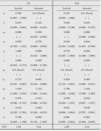
4.2.1 Assessing the fit of the model to inflation persistence: 15 moments
First, we examine the performance of the two models for fitting the GI data (see Table 2). As long as the profit maximizing rule (or purely forward-looking) determines the total amount of the output in the economy, the inflation dynamics are primarily captured by inherited and extrinsic persistence. Indeed, the model of purely forward-looking behavior has much higher estimated values for the parametersκand
ρπ than its hybrid variant; i.e. bκ: 0.12 (forward)>0.05 (hybrid), ρbπ: 0.51 (forward)>0.0 (hybrid).
Table 2: Parameter estimates for inflation persistence with 15 moments
GI GM
hybrid forward hybrid forward
α 0.768 0.0 (fixed) 0.105 0.0 (fixed)
(0.007 - 1.000) ( - ) (0.000 - 1.000) ( - )
κ 0.047 0.123 0.052 0.058
(0.009 - 0.084) (0.000 - 0.318) (0.000 - 0.136) (0.008 - 0.107)
ρπ 0.000 0.506 0.000 0.086
( - ) (0.078 - 0.933) ( - ) (0.000 - 0.269)
σπ 0.679 0.778 0.638 0.644
(0.103 - 1.255) (0.603 - 0.952) (0.454 - 0.823) (0.491 - 0.798)
χ 1.000 0.999 0.774 0.802
( - ) (0.441 - 1.000) (0.497 - 1.000) (0.499 - 1.000)
τ 0.094 0.089 0.000 0.000
(0.015 - 0.174) (0.000 - 0.192) ( - ) ( - )
ρx 0.0 (fixed) 0.0 (fixed) 0.0 (fixed) 0.0 (fixed)
( - ) ( - ) ( - ) ( - )
σx 0.727 0.662 0.404 0.369
(0.547 - 0.907) (0.416 - 0.909) (0.118 - 0.691) (0.068 - 0.671)
φπ 1.659 1.744 1.798 1.943
(1.000 - 2.334) (1.084 - 2.404) (1.000 - 4.039) (1.000 - 4.465)
φx 0.378 0.181 0.729 0.652
(0.026 - 0.731) (0.000 - 0.452) (0.226 - 1.231) (0.087 - 1.217)
φr 0.544 0.463 0.841 0.849
(0.323 - 0.765) (0.248 - 0.678) (0.698 - 0.984) (0.707 - 0.991)
σr 0.786 0.662 0.391 0.384
(0.382 - 1.190) (0.155 - 1.169) (0.099 - 0.684) (0.080 - 0.688)
J(θ) 1.30 3.24 2.26 2.44
Note: The discount factor parameterβis calibrated to 0.99. The 95% asymptotic confidence intervals are given
in brackets.
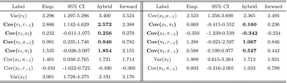
This finding is shown in Table 3. In particular, the results show that the hybrid variant of the model can approximate the inflation dynamics better than the other; e.g. see Cov(rt, xt−k), Cov(xt, πt−k),
Cov(πt, rt−k). Nevertheless, the fit of the nested model is not so bad, because the estimated values of
auto- and crosscovariances at lag 1 lie within the 95% confidence intervals of the empirical moments. Note here that we do not aim to match the auto- and cross-covariances up to higher lags; this will be discussed later.
simulated 1% and 5% criteria are 0.51 and 0.27, respectively; see the right panel of Figure 3 in appendix F. Therefore the null hypothesis cannot be rejected.
Table 3: Empirical and model-generated moments for inflation persistence: 15 moment conditions
Label Emp. 95% CI hybrid forward Label Emp. 95% CI hybrid forward
Var(rt) 3.296 1.297-5.296 3.400 3.524 Cov(xt,x−1) 2.523 1.356-3.690 2.365 2.495 Cov(rt, r−1) 2.886 1.142-4.629 2.572 2.388 Cov(xt, πt) 0.069 -0.415-0.552 0.160 0.236 Cov(rt, xt) 0.232 -0.611-1.075 0.256 0.270 Cov(xt, π−1) -0.350 -1.239-0.539 -0.342 -0.234 Cov(rt, x−1) 0.991 0.235-1.746 0.946 0.782 Cov(πt, r−1) 1.288 -0.021-2.597 1.067 0.846
Cov(rt, πt) 1.535 -0.026-3.097 1.854 2.155 Cov(πt, x−1) 0.588 0.199-0.977 0.527 0.442
Cov(xt, π−1) 1.401 0.038-2.765 1.731 1.714 Var(πt) 1.989 0.615-3.364 1.713 1.921 Cov(xt, r−1) -0.450 -1.622-0.722 -0.490 -0.369 Cov(πt, π−1) 0.893 -0.216-2.001 1.033 0.789
Var(xt) 3.001 1.728-4.275 3.191 3.176
Note: 95% CI means the 95% asymptotic confidence intervals for empirical moments.
To save space, we do not report the model-generated moments for GM. Indeed, when we compare trajectories of the model-generated moments (i.e. hybrid and forward), the model covariance profiles almost overlap with each other. The two models provide a good fit to auto- and cross-covarainces at the short lag. More ambitious attempts to take the model to data will be discussed using alternative moment conditions later, because the model has a bad fit to the ones up to relatively large lags (two or three years).
4.2.2 Assessing the fit of the model to the output gap persistence: 15 moments
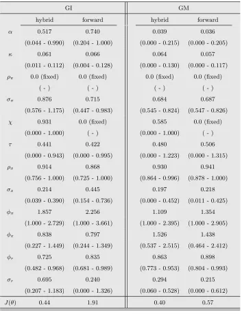
The estimated parameters for the model with or without a habit formation are displayed in Table 4; in the purely forward-looking behavior,χ is set to zero, whereas this parameter is subject to the estimation in the hybrid variant of the model. The MM estimates of the two models have almost similar values except for the degree of the supply shock (σx) and the Taylor rule coefficient (φπ).
It can be seen from the GI data that the estimated value for the supply shocks with the model of an optimal consumer behavior is two times higher than the parameter value of the other model (bσx: 0.45
(forward)> 0.21 (hybrid)). This implies that the output gap dynamics are more or less driven by the high level of the supply shocks when a simple rule of thumb behavior is not allowed in the IS equation. As a result, the persistence from the supply shocks is transmitted to inflation, which is indicated by a lower value for the estimated price indexation parameter; i.e. αb: 0.517 (hybrid) < 0.740 (forward). Further, concerning the model, which allows a fraction of consumers to have a rule of thumb behavior, the estimation results indicate a low value for the monetary coefficients on the inflation gap; i.e. φbπ:
Table 4: Parameter estimates for the output gap persistence with 15 moments
GI GM
hybrid forward hybrid forward
α 0.517 0.740 0.039 0.036
(0.044 - 0.990) (0.204 - 1.000) (0.000 - 0.215) (0.000 - 0.205)
κ 0.061 0.066 0.064 0.057
(0.011 - 0.112) (0.004 - 0.128) (0.000 - 0.130) (0.000 - 0.117)
ρπ 0.0 (fixed) 0.0 (fixed) 0.0 (fixed) 0.0 (fixed)
( - ) ( - ) ( - ) ( - )
σπ 0.876 0.715 0.684 0.687
(0.576 - 1.175) (0.447 - 0.983) (0.545 - 0.824) (0.547 - 0.826)
χ 0.931 0.0 (fixed) 0.585 0.0 (fixed)
(0.000 - 1.000) ( - ) (0.000 - 1.000) ( - )
τ 0.441 0.422 0.480 0.506
(0.000 - 0.943) (0.000 - 0.995) (0.000 - 1.223) (0.000 - 1.315)
ρx 0.914 0.868 0.930 0.941
(0.756 - 1.000) (0.725 - 1.000) (0.864 - 0.996) (0.878 - 1.000)
σx 0.214 0.445 0.197 0.218
(0.039 - 0.390) (0.154 - 0.736) (0.000 - 0.452) (0.011 - 0.425)
φπ 1.857 2.256 1.109 1.354
(1.000 - 2.729) (1.000 - 3.661) (1.000 - 2.395) (1.000 - 2.905)
φx 0.838 0.797 1.526 1.438
(0.227 - 1.449) (0.244 - 1.349) (0.537 - 2.515) (0.464 - 2.412)
φr 0.725 0.835 0.863 0.898
(0.482 - 0.968) (0.681 - 0.989) (0.773 - 0.953) (0.804 - 0.993)
σr 0.695 0.240 0.294 0.215
(0.207 - 1.183) (0.000 - 1.326) (0.060 - 0.528) (0.000 - 0.612)
J(θ) 0.44 1.91 0.40 0.57
Note: The discount factor parameterβis calibrated to 0.99. The 95% asymptotic confidence intervals are given in brackets.
Now, we use the loss function values to provide a formal test to the two specifications in the IS equation. In GI, these values are respectively 0.44 and 1.91 for the model with and without habit formation. The simulated 1% and 5% test criteria are 1.89 and 1.08, respectively; see the left panel of Figure 4. Since the estimated value for QLR exceeds the criterion at the 5% level, we reject the null hypothesis that the two models are equivalent. This implies that the output gap dynamics are better approximated by the consumption behavior in a rule of thumb manner. This finding is shown in Table 5. For instance, the covariance profiles of (rt, xt−k), (xt, xt−k), and (πt, πt−k) are better captured by the hybrid variant of
the model.
1% and 5% test criteria are 7.58 and 12.37, respectively; see the right panel of Figure 4 in appendix F. We cannot reject the null hypothesis that the two models are equivalent. To save space, we do not report the model-generalted moments for the GM period; the covariance profiles from the two models more or less overlap with each other.
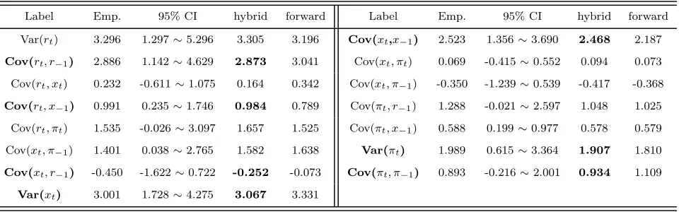
Table 5: Empirical and model-generated moments for the output gap persistence: 15 moment conditions
Label Emp. 95% CI hybrid forward Label Emp. 95% CI hybrid forward
Var(rt) 3.296 1.297∼5.296 3.305 3.196 Cov(xt,x−1) 2.523 1.356∼3.690 2.468 2.187 Cov(rt, r−1) 2.886 1.142∼4.629 2.873 3.041 Cov(xt, πt) 0.069 -0.415∼0.552 0.094 0.073
Cov(rt, xt) 0.232 -0.611∼1.075 0.164 0.342 Cov(xt, π−1) -0.350 -1.239∼0.539 -0.417 -0.368 Cov(rt, x−1) 0.991 0.235∼1.746 0.984 0.789 Cov(πt, r−1) 1.288 -0.021∼2.597 1.048 1.025
Cov(rt, πt) 1.535 -0.026∼3.097 1.657 1.525 Cov(πt, x−1) 0.588 0.199∼0.977 0.578 0.579
Cov(xt, π−1) 1.401 0.038∼2.765 1.582 1.638 Var(πt) 1.989 0.615∼3.364 1.907 1.810
Cov(xt, r−1) -0.450 -1.622∼0.722 -0.252 -0.073 Cov(πt, π−1) 0.893 -0.216∼2.001 0.934 1.109 Var(xt) 3.001 1.728∼4.275 3.067 3.331
Note: 95% CI means the 95% asymptotic confidence intervals for empirical moments.
4.3
Basic results on the maximum likelihood estimation
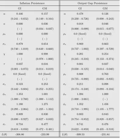
For comparison purposes, we present the ML estimates of the NKM, because it is often uncommon to see that the MM estimation includes all relevant information about the DGP; the MM estimation is likely to be as efficient as ML when the chosen moment conditions encompass as many features of the data as possible. Table 6 shows that ML and MM give somewhat similar parameter estimates to the hybrid variant of the model for inflation persistence. For instance, the parameter estimates for the price indexation α
are 0.45 and 0.16 for the GI and GM data, respectively. The ML estimates also support the existence of intrinsic inflation persistence in the model. In other words, a rule of thumb behavior in the price-setting rule accounts for inflation persistence. Moreover, the ML estimation gives a very small value for the slope of the Phillips curve (bκ= 0.0 (GI) and 0.04 (GM)). This implies that individual firms are less responsive to changes in economic activity (i.e., the Phillips curve is flat). Hence, inflation dynamics in GI are primarily driven by intrinsic (moderate) and extrinsic (strong) persistence; i.e. αb: 0.446,bσπ: 0.879.
In comparison, we find a slight difference for the estimation of the output gap persistence. For instance, the comparison of the estimation results between ML and MM shows that MM gives a much lower value for the habit formation parameter (χ=0.28 and 0.25 for the GI and GM data). Further interesting observation from Table 6 is that the ML estimates for the intertemporal elasticity of substitution is found to be much lower (τ=0.08 and 0.03 for the GI and GM data). This implies that intrinsic persistence in the output gap dynamics is less affected by the substitution effects implied by the Fisher equation.
choice for evaluating the model’s goodnese-of-fit to the data; the moment matching results in a closer fit to the sample autocovariance. The statistical efficiency and consistency of the parameter estimation used in this study will be investigated via a Monte Carlo study later.
Table 6: ML estimates for inflation and the output gap persistence
Inflation Persistence Output Gap Persistence
GI GM GI GM
α 0.446 0.157 α 0.478 0.126
(0.241 - 0.652) (0.149 - 0.164) (0.230 - 0.726) (0.008 - 0.243)
κ 0.000 0.036 κ 0.018 0.046
( - ) (0.034 - 0.037) (0.000 - 0.099) (0.015 - 0.077)
ρπ 0.000 0.000 ρπ 0.0 (fixed) 0.0 (fixed)
( - ) ( - ) ( - ) ( - )
σπ 0.879 0.654 σπ 0.869 0.663
(0.740 - 1.019) (0.649 - 0.660) (0.737 - 1.002) (0.597 - 0.729)
χ 1.000 0.998 χ 0.281 0.254
( - ) (0.978 - 1.000) (0.245 - 0.316) (0.133 - 0.374)
τ 0.037 0.016 τ 0.081 0.027
(0.001 - 0.073) (0.014 - 0.019) (0.038 - 0.125) (0.014 - 0.040)
ρx 0.0 (fixed) 0.0 (fixed) ρx 0.808 0.763
( - ) ( - ) (0.735 - 0.880) (0.692 - 0.835)
σx 0.523 0.253 σx 0.211 0.098
(0.442 - 0.604) (0.252 - 0.255) (0.174 - 0.248) (0.093 - 0.104)
φπ 1.353 1.001 φπ 1.394 1.000
(1.000 - 2.760) (1.000 - 1.112) (1.000 - 2.661) ( - )
φx 1.180 1.275 φx 1.352 1.456
(0.295 - 2.064) (1.225 - 1.324) (0.710 - 1.995) (1.135 - 1.777)
φr 0.809 0.830 φr 0.803 0.843
(0.690 - 0.927) (0.827 - 0.833) (0.754 - 0.852) (0.828 - 0.857)
σr 0.734 0.477 σr 0.741 0.476
(0.618 - 0.850) (0.472 - 0.481) (0.622 - 0.859) (0.435 - 0.518)
L(θ) -308.86 -233.99 L(θ) -309.53 -231.84
Note: The discount factor parameterβis calibrated to 0.99. The 95% asymptotic confidence intervals are given in brackets.
the unique minimum points.
To make a more systemic investigation on our choice of moments in the model estimation, the next section examines the parameter estimates of the model using a large set of moment conditions.
4.4
Validity of extra moment conditions
In this section, we assess the sensitivity of the MM estimates to the changes in moment conditions. From this investigation, we will find that alternative moment conditions do not induce qualitative changes in the parameter estimation. To make our choice of moment condtions more reliable, first we present the vector autoregressive (VAR) model with lag 4 as a reference model; see appendix C for optimal lag selection criteria. Then we examine the persistence of the key macro data in the U.S. economy using auto- and cross-covariances up to lag 4.
4.4.1 Assessing the fit of the model to inflation persistence: 42 moments
With alternative moment conditions in hand (42 moments), we now estimate two specifications of the NKM: forward-looking (α = 0) and hybrid case (i.e. α is a free parameter). Table 7 shows that the parameter estimates speak for strong backward-looking behavior in the NKM. And the MM estimates with a small and large set of moments give qualitatively similar values except for the policy shock parameter (σr=0.0). Indeed, ML would avoid such an estimate, given that there is a stochastic singularity with zero
policy shock (i.e., the likelihood value becomes negative infinity at this point).
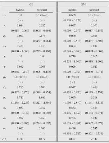
Next, we turn our attention to the model comparison. In the GI data, we found that the price indexation parameter is a corner solution. Accordingly we treatα as being exogenously fixed at unity, because HMT assume that the estimated parameters are in the interior of the admissible region (see their assumption 2.5 (b)). Put differently, since the price indexation parameter is set to different values, it can be seen that two models are now equally accurate and identical in population. In this respect, we treat two models as being overlapping and apply a two step sequential test for model comparison. On the contrary, a value for the estimated price indexation parameter lies in the interior of the parameter space for fitting the GM data (α= 0.525). In this case, the hybrid version of the model nests the one with the purely forward-looking expectations.
In the period of GI, the hybrid variant of NKP has a better goodness-of-fit to the data (J = 11.93) than the purely forward-looking version of the model (J = 42.77). Indeed, the AR (1) coefficient for the cost push shock (ρπ) plays an important role in the purely forward-looking NKP (see Table 7).9 The
results also show that inherited persistence has a significant impact on the output gap dynamics in the hybrid-variant of the model (bκ= 0.044).
9
The estimated value for the parameterσr hit the boundary. This makes the objective function ill-behaved and partial derivatives numerically unstable. We set it to zero and compute the numerical derivatives of the other parameters for the
In order to examine the significant difference of moment estimates between the two specifications, we substract the objective function value of purely forward-looking NKM from the one of hybrid variant; i.e. QLR = 30.83. The difference exceeds the simulated criterion (95%) of the χ2-type distribution in
[image:20.595.127.478.232.689.2]the model comparison. According to the simulated test distribution, critical values for the 99% and 95% confidence intervals are 16.99 and 9.96 respectively (see the left panel of Figure 5 in appendix F). Since the test statistic exceeds the critical value at the 5% level, we proceed to take the second step of model comparison, which asymptotically examines the validity of the goodness-of-fit.
Table 7: Parameter estimates for inflation persistence with 42 moments
GI GM
hybrid forward hybrid forward
α 1.0 0.0 (fixed) 0.509 0.0 (fixed)
( - ) ( - ) (0.126 - 0.924) ( - )
κ 0.044 0.155 0.037 0.102
(0.018 - 0.069) (0.000 - 0.395) (0.000 - 0.075) (0.017 - 0.187)
ρπ 0.000 0.675 0.000 0.596
( - ) (0.387 - 0.964) (0.000 - 0.813) (0.367 - 0.825)
σπ 0.470 0.518 0.364 0.231
(0.000 - 1.686) (0.233 - 0.790) (0.048 - 0.680) (0.093 - 0.369)
χ 1.0 1.0 0.770 0.915
( - ) ( - ) (0.515 - 1.000) (0.518 - 1.000)
τ 0.092 0.063 0.020 0.027
(0.045 - 0.140) (0.008 - 0.118) (0.000 - 0.055) (0.000 - 0.074)
ρx 0.0 (fixed) 0.0 (fixed) 0.0 (fixed) 0.0 (fixed)
( - ) ( - ) ( - ) ( - )
σx 0.716 0.600 0.547 0.468
(0.462 - 0.970) (0.348 - 0.853) (0.202 - 0.820) (0.185 - 0.751)
φπ 1.740 1.809 2.025 2.218
(1.255 - 2.225) (1.221 - 2.397) (1.000 - 2.870) (1.141 - 3.114)
φx 0.080 0.157 0.563 0.564
(0.000 - 0.542) (0.000 - 0.528) (0.216 - 1.059) (0.154 - 0.974)
φr 0.267 0.458 0.765 0.732
(0.000 - 0.905) (0.224 - 0.692) (0.619 - 0.881) (0.592 - 0.872)
σr 0.000 0.000 0.486 0.545
( - ) ( - ) (0.303 - 0.727) (0.351 - 0.739)
J(θ) 11.93 42.77 23.97 27.47
Note: The discount factor parameterβis calibrated to 0.99. The 95% asymptotic confidence intervals are given in brackets.
null hypothesis, the test static follows a standard normal distribution; i.e. √T·QLR(θA, θB)∼N(0, w2 0).
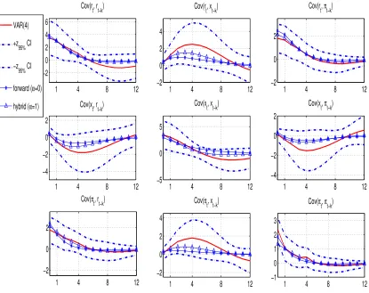
The estimate of√T·QLR/wbis 1.37, which is smaller than a critical value at the 5% significance level of the two-tailed test. Therefore the results show that both models have the same goodness-of-fit and the null hypothesis cannot be rejected.10 Figure 1 presents the model-generated moment conditions at three
years for GI and contrasts them with the empirical estimates using a VAR (4) process.
1 4 8 12
−2 0 2 4 6 Cov(r t, rt−k)
1 4 8 12
−2 0 2 4
Cov(r t, xt−k)
1 4 8 12
−2 0 2
Cov(r t, πt−k)
1 4 8 12
−4 −2 0 2
Cov(x t, rt−k)
1 4 8 12
−5 0 5
Cov(x t, xt−k)
1 4 8 12
−4 −2 0 2
Cov(x t, πt−k)
1 4 8 12
−2 0 2
Cov(π t, rt−k)
1 4 8 12
−2 0 2 4
Cov(π t, xt−k)
1 4 8 12
−1 0 1 2 3 Cov(π t, πt−k) VAR(4)
+z 95% CI
−z 95% CI
forward (α=0)
[image:21.595.78.493.179.508.2]hybrid (α=1)
Figure 1: Covariance profiles for inflation persistence in GI (dashed: empirical,△: hybrid, *: forward)
Note: The empirical auto- and cross-covariances are computed using an unrestricted fourth-order vector
au-toregression (VAR) model. The asymptotic 95% confidence bands are constructed following Coenen (2005).
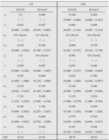
In the period of GM (Table 7), it is shown that the hybrid variant of NKP fits the data better (23.97). The estimation results indicate high values for the inherited and extrinsic persistence in the model of purely forward-looking behavior, because these can offset the impact of inherited persistence on the output gap dynamics; i.e. κb: 0.102 (forward) >0.037 (hybrid), ρbπ: 0.596 (forward)> 0.0 (hybrid). However, the
other parameter estimates are not different in both specifications.
10
This statistical inference does not remain the same if the price indexation parameter is allowed to exceed unity. The
1 4 8 12 −2
0 2
Cov(r
t, rt−k)
1 4 8 12
−1 0 1
Cov(r
t, xt−k)
1 4 8 12
−0.5 0 0.5
Cov(r
t, πt−k)
1 4 8 12
−1 0 1
Cov(x
t, rt−k)
1 4 8 12
−1 0 1 2
Cov(xt, xt−k)
1 4 8 12
−0.5 0 0.5
Cov(x
t, πt−k)
1 4 8 12
−0.5 0 0.5
Cov(πt, r
t−k)
1 4 8 12
−0.5 0 0.5
Cov(πt, x
t−k)
1 4 8 12
−0.5 0 0.5 1
Cov(πt, πt−k) VAR(4)
+z
95% CI
−z
95% CI
[image:22.595.77.493.80.413.2]forward (α=0) hybrid (α=0.51)
Figure 2: Covariance profiles for inflation persistence in GM (dashed: empirical,△: hybrid, *: forward)
Note: The empirical auto- and cross-covariances are computed using an unrestricted fourth-order vector
au-toregression (VAR) model. The asymptotic 95% confidence bands are constructed following Coenen (2005).
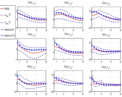
4.4.2 Assessing the fit of the model to the output gap persistence: 42 moments
Table 8 shows the MM estimates for the output gap persistence using alternative moment conditions. Note here that the intertemporal elasticity of substitution of the both models has high estimated values in the GI and GM data; all the estimated values forρxexceed 0.7. In GI, this value increases substantially in
[image:23.595.126.479.220.672.2]the model with purely forward-looking expectations, which can cover the absence of intrinsic persistence in the IS equation; i.e. χ=0.0 (fixed),τb= 0.676.
Table 8: Parameter estimates for the output gap persistence with 42 moments
GI GM
hybrid forward hybrid forward
α 1.0 0.998 0.186 0.203
( - ) ( - ) (0.000 - 0.396) (0.000 - 0.441)
κ 0.054 0.037 0.086 0.088
(0.005 - 0.102) (0.010 - 0.065) (0.037 - 0.134) (0.027 - 0.149)
ρπ 0.0 (fixed) 0.0 (fixed) 0.0 (fixed) 0.0 (fixed)
( - ) ( - ) ( - ) ( - )
σπ 0.519 0.428 0.609 0.579
(0.099 - 0.939) (0.108 - 0.747) (0.461 - 0.757) (0.410 - 0.749)
χ 1.0 0.0 (fixed) 0.991 0.0 (fixed)
( - ) ( - ) ( - ) ( - )
τ 0.205 0.676 0.237 0.236
(0.000 - 0.436) (0.000 - 1.897) (0.000 - 0.547) (0.000 - 0.803)
ρx 0.707 0.890 0.854 0.790
(0.290 - 1.000) (0.743 - 1.000) (0.686 - 1.000) (0.583 - 0.997)
σx 0.213 0.519 0.140 0.340
(0.016 - 0.410) (0.169 - 0.869) (0.000 - 0.298) (0.037 - 0.642)
φπ 1.741 2.046 2.133 2.224
(1.154 - 2.327) (1.000 - 3.134) (1.000 - 3.279) (1.000 - 3.764)
φx 0.169 1.103 0.762 0.588
(0.000 - 0.584) (0.275 - 1.931) (0.189 - 1.335) (0.000 - 1.202)
φr 0.389 0.889 0.770 0.783
(0.000 - 0.853) (0.753 - 1.026) (0.640 - 0.900) (0.648 - 0.917)
σr 0.012 0.016 0.447 0.448
( - ) ( - ) (0.248 - 0.645) (0.212 - 0.685)
J(θ) 10.54 31.64 20.79 23.85
Note: The discount factor parameterβis calibrated to 0.99. The 95% asymptotic confidence intervals are given in brackets.
data, which strengthens a rule of thumb behavior in consumption. This implies that the rule of thumb behavior reinforces the degree of endogenous persistence in the output gap dynamics. However, as long as the model predicts that households behave optimally (i.e. without a simple rule of thumb behavior,
χ= 0), the result indicates the strong degree of the supply shocks; the estimated value is more than twice as high as the one of the hybrid model; i.e. bσx: 0.519 (forward)>0.213 (hybrid) for GI, 0.340 (forward) >0.140 (hybrid) for GM).
As for the GI data, we treat the two models as being overlapping, because the habit formation param-eter is now a corner solution. In the first step of the model comparison, we compare the objective function values (QLR = 21.10). The simulated 5% and 1% criteria are 19.63 and 34.59 respectively (see the left panel of Figure 6 in appendix F). Since the estimated QLR exceeds the 5% criterion value for the model comparison, we support the hypothesis that two models have different moments. In the second step, we estimate √T ·QLR/wb of which value is 1.02. However, this value does not exceed the criterion in the standard normal distribution. As a result, we conclude that there is no significant difference between two models in macthing the empirical moments; i.e. the two models have different moments, but an equivalent fit to the empirical moments. To save space, we do not provide the model covariance profiles for the output gap persistence. Note here that the result of the MM estimates with a large set of moments provides a closer fit (i.e. the sample auto- and cross-covariances up to large lags).
5
Attaining efficiency from moment conditions
In this section we study the finite sample properties of MM and ML; we investigate the role of model misspecification in the bias of the parameter estimation. Further, we discuss the empirical performance of model selection methods using the Akaike’s and the Bayesian information criterion.
5.1
Monte Carlo study
The Monte Carlo (MC) experiment attempts to clearly demonstrate the statistical efficiency of the estima-tion methods, which are used in the previous secestima-tion. Besides, we aim to investigate the role of the choice of moments and its influence on the parameter estimates. To begin, we consider the model specification of inflation persistence and set the parameters near to the values obtained by the MM estimation with 15 moments (see Table 2): e.g. high degree of backward-looking behavior (α=0.750), moderate inherited persistence (κ=0.050), and no extrinsic persistence (ρπ=0.0). Next, we generate 1,000 time series each
consisting of 550 observations. The first 50 observations are removed as a transient period. Three sample sizes are considerd: 100, 200, and 500. We use the Matlab R2010a for this MC study As for the opti-mization routine, we use the unconstrained miniopti-mization"fminicon"with the algorithm ’interior-point’; maximum iteration and tolerance level are set to 500 and 10−6respectively.
We conduct the MC experiments by considering two cases of model specification; i.e. correctly specified and misspecified. For the former, we discuss the finite sample properties of the MM and ML estimation. Turning to the misspecified case, we consider the model with purely forward-looking expecations and examine the degree of bias in the parameter estimates; i.e. (1) to what extent the extrinsic persistence (ρπ) is inflated due to the misspecification and (2) how much the model misspecification affects the
estimates for other strucutral parameters.
The main findings for the correctly specified case in Table 9 can be summarized as follows:
• For both ML and MM, the estimate of the price indexation paramterαis downward-biased, whereas the AR (1) coefficient of inflation shocks is estimated to be positive.
• ML has slightly poorer finite sample properties than MM. This implies that conventional Gaussian asymptotic approximation to the sample distribution is not as much precise as MM, as long as the sample size is small.
• The asymptotic efficiency of the ML estimates appears superior to MM, since the the mean of standard errors over 1000 estimations shows that the confidence intervals for the MM estimates are noticeably narrow. However, the large sample size remarkably improves the asymptotic efficiency of the MM estimates; e.g. T=500.
for large uncertainty in the estimates of other structural parameters; in other words, incorporating more second moments in the objective function improves the fit of the model to the persistence of inflation dynamics, but reduces efficiency in the estimates of other parameters.
• Another point, which is worthwhile to mention, is that we obtain the large asymptotic error for the policy shock parameterσr; S.E : 1.407 for T=100. This is attributed to the fact that the estimated
values sometimes hit the boundary (i.e. σr= 0.0), which makes the numerical derivative unstable.
This problem does not occur in the case where the large sample size is used (e.g. T=500).
With regard to the misspecified case, the MC results exhibit the high correlation between the price indexation and AR (1) coefficient of the inflation shocks; see appendix G. Indeed, it is shown in Table G.2 that the AR (1) coefficient is strongly upward-biased for both MM and ML, of which estimates offset the effects of intrinsic persistence on the inflation dynamics; e.g. ρπ: 0.616 (ML), 0.632 (MM with 15
moments), 0.598 (MM with 42 moments) when the sample size is 100. The large sample size does not correct the bias of this parameter.
Similarly, the degree of the inflation shockσπ is more or less downward-biased. In addition, the slope
Table 9: Monte Carlo results on the MM and ML estimates, ( ): root-mean-square-error, S.E : mean of standard error
ML MM with 15 moments MM with 42 moments
θ0
T = 100 T = 200 T = 500 T = 100 T = 200 T = 500 T = 100 T = 200 T = 500
α 0.750 0.523 (0.375) 0.573 (0.322) 0.651 (0.228) 0.614 (0.256) 0.654 (0.196) 0.692 (0.121) 0.700 (0.245) 0.702 (0.205) 0.729 (0.118) S.E : 0.162 S.E : 0.170 S.E : 0.175 S.E : 0.319 S.E : 0.222 S.E : 0.138 S.E : 0.281 S.E : 0.190 S.E : 0.113
κ 0.050 0.074 (0.076) 0.066 (0.081) 0.056 (0.014) 0.083 (0.057) 0.068 (0.030) 0.058 (0.015) 0.093 (0.075) 0.073 (0.042) 0.058 (0.018) S.E : 0.054 S.E : 0.048 S.E : 0.041 S.E : 0.042 S.E : 0.025 S.E : 0.013 S.E : 0.050 S.E : 0.030 S.E : 0.014
ρπ 0.000 0.218 (0.330) 0.172 (0.284) 0.097 (0.198) 0.175 (0.255) 0.129 (0.194) 0.082 (0.124) 0.194 (0.299) 0.147 (0.241) 0.078 (0.144) S.E : 0.112 S.E : 0.1000 S.E : 0.076 S.E : 0.327 S.E : 0.238 S.E : 0.152 S.E : 0.313 S.E : 0.230 S.E : 0.150
σπ 0.675 0.602 (0.330) 0.619 (0.125) 0.640 (0.073) 0.613 (0.113) 0.624 (0.085) 0.639 (0.056) 0.564 (0.1778) 0.584 (0.136) 0.618 (0.088) S.E : 0.044 S.E : 0.047 S.E : 0.048 S.E : 0.143 S.E : 0.106 S.E : 0.068 S.E : 0.172 S.E : 0.130 S.E : 0.086
χ 1.000 0.935 (0.113) 0.949 (0.090) 0.967 (0.053) 0.932 (0.108) 0.948 (0.078) 0.962 (0.055) 0.941 (0.075) 0.956 (0.083) 0.966 (0.059) S.E : 0.159 S.E : 0.183 S.E : 0.201 S.E : 0.173 S.E : 0.126 S.E : 0.082 S.E : 0.207 S.E : 0.151 S.E : 0.098
τ 0.090 0.089 (0.031) 0.088 (0.023) 0.087 (0.014) 0.101 (0.039) 0.095 (0.026) 0.091 (0.016) 0.105 (0.044) 0.097 (0.030) 0.092 (0.018) S.E : 0.045 S.E : 0.047 S.E : 0.048 S.E : 0.040 S.E : 0.028 S.E : 0.017 S.E : 0.041 S.E : 0.029 S.E : 0.018
σx 0.700 0.695 (0.059) 0.697 (0.043) 0.699 (0.025) 0.743 (0.102) 0.735 (0.073) 0.724 (0.048) 0.738 (0.123) 0.729 (0.086) 0.721 (0.054) S.E : 0.050 S.E : 0.052 S.E : 0.053 S.E : 0.086 S.E : 0.062 S.E : 0.039 S.E : 0.121 S.E : 0.089 S.E : 0.057
φπ 1.650 1.666 (0.183) 1.654 (0.118) 1.652 (0.074) 1.681 (0.194) 1.664 (0.123) 1.659 (0.076) 1.705 (0.229) 1.679 (0.145) 1.665 (0.088) S.E : 0.345 S.E : 0.316 S.E : 0.274 S.E : 0.210 S.E : 0.147 S.E : 0.093 S.E : 0.214 S.E : 0.151 S.E : 0.098
φx 0.375 0.362 (0.124) 0.361 (0.083) 0.366 (0.052) 0.337 (0.148) 0.343 (0.100) 0.352 (0.063) 0.294 (0.191) 0.317 (0.129) 0.344 (0.082) S.E : 0.227 S.E : 0.224 S.E : 0.228 S.E : 0.137 S.E : 0.097 S.E : 0.062 S.E : 0.156 S.E : 0.110 S.E : 0.071
φr 0.550 0.543 (0.048) 0.545 (0.034) 0.547 (0.021) 0.525 (0.063) 0.531 (0.045) 0.538 (0.027) 0.524 (0.080) 0.532 (0.056) 0.542 (0.034) S.E : 0.068 S.E : 0.070 S.E : 0.077 S.E : 0.074 S.E : 0.052 S.E : 0.033 S.E : 0.086 S.E : 0.061 S.E : 0.039
σr 0.750 0.738 (0.056) 0.743 (0.038) 0.748 (0.024) 0.723 (0.087) 0.736 (0.057) 0.746 (0.034) 0.617 (0.269) 0.672 (0.173) 0.721 (0.053) S.E : 0.053 S.E : 0.055 S.E : 0.056 S.E : 0.109 S.E : 0.076 S.E : 0.048 S.E : 1.407 S.E : 0.675 S.E : 0.087
L(θ) orJ(θ) -385.76 -800.93 -2015.15 0.30 0.25 0.23 7.55 5.84 4.92
2
5.2
Model selection and discussion
[image:28.595.125.478.225.340.2]From the empirical investigation on the MM estimates with a large set of moments, we found that the statistical power of the model comparison test is weak and the result becomes inconclusive; here we treat two models as being overlapping. Note here that we use the small sample to estimate the parameters of the NKM in which the asymptotic test of the model comparison is likely to make a Type II error; i.e. we accept the null hypothesis when the equal fit of moments is false.11
Table 10: Model selection using information criteria: inflation persistence GI (T=78) GM (T=99) ML hybrid forward ML hybrid forward
L(θ)/T -3.96 -4.41 -4.82 -2.36 -2.69 -2.69 AIC 8.20 9.02 9.90 4.95 5.61 5.58 BIC 8.53 9.43 10.20 5.24 5.90 5.84
Ranking 1 2 3 1 3 2
Note: The backward- and forward-looking behaviors are examined using auto- and cross-covariances
at lag 1.
To make the formal test more elaborate, we rank the model according to the well-known information criteria in the ML estimation. For this purpose, we suppose that the MM parameter estimates are possible solutions in the likelihood function. Table 10 and 11 report the mean value for the log-likelihood and the model selection criterion; the case of inflation and the output gap persistence respectively. Note here that we only present MM with a small set of the moment conditions (auto- and cross-covarainces at lag 1), because MM with alternative moments (auto- and cross-covarainces at lag 4) yields the zero policy shock for the GI data.
According to AIC and BIC, by definition, the ML estimates are preferred for both GI and GM data. If the assumption of normality is not violated and the model is correctly specified, we believe that the parameter estimates of the ML estimator are the most efficient; this statistical inference is verified by the MC study in the previous section. Nevertheless, the values for AIC and BIC using the MM estimation do not differ too much. This implies that matching the auto- and cross-covarainces at lag 1 provide more or less the same efficiency as the ML approach. Also the statistical inference for the expectation formation process does not change; i.e. the hybrid variant of the model can approximate inflation and the output gap dynamics better than the model with forward-looking behavior for fitting the GI data. On the other hand, the inconclusive result for the GM data shows that the model with forward-looking expectations of the price-setting rule is preferred due to its parsimonious description of the data.
11
Marmer and Otsu (2012) studied the general optimality of comparison of misspecified models and proposed a feasible
Table 11: Model selection using information criteria: the output gap persistence GI (T=78) GM (T=99)
ML hybrid forward ML hybrid forward
L(θ)/T -3.97 -4.62 -7.88 -2.34 -3.09 -4.22 AIC 8.22 9.51 16.01 4.91 6.41 8.64 BIC 8.55 9.85 16.31 5.19 6.69 8.90
Ranking 1 2 3 1 2 3
Note: The backward- and forward-looking behaviors are examined using auto- and cross-covariances
at lag 1.
6
Conclusion
This paper considered the structural estimation and model selection for expectation formation process in the NKM. We examined the importance of the future expected and lagged values in the inflation and output dynamics using US data; i.e. forward- and backward-looking expectations in the NKPC and the IS equation. The models are estimated by the classical estimation methods of MM and ML. In the former, we derived the analytical form of the auto- and cross-covariances in a linear system of the NKM; we estimate the parameters of the NKM by matching the model-generated moments with their empirical counterparts. These empirical findings are compared with the ones obtained by the ML estimation while their sensitivity to the moment conditions is also exmained.
According to the estimated loss function values obtained by MM, we evaluated two competing models using the formal test of HMT when they are overlapping or one model is nested within another. The results obtained with the GI and GM data show that the empirical performance of the NKM can be improved when allowing for backward-looking expectations in the NKP and the IS equation. After all, the backward-looking behavior in the NKM plays an important role in approximating inflation and the output gap dynamics in the DGP. This result suggests intrinsic persistence as the main source of inflation and the output gap dynamics in the GI data. However, we cannot reject the null hypothesis at the 5% level, because the model with purely forward-looking expecations and its hybrid-variant in the NKPC and IS equation have an equal fit to the GM data. These empirical findings are verified using the MC experiments; we investigated the statistical efficiency of the estimators and the implications for the model selection.
References
Altonji, J. and Segal, L. (1996): Small-sample bias in GMM estimation of covariance structures.
Journal of Business and Economic Statistics, 14, 353–366.
Amato, J.D. and Laubach, T. (2003): Rule-of-thumb behaviour and monetary policy. European
Economic Review, Vol. 47(5), pp. 791–831.
Amato, J.D. and Laubach, T. (2004): Implications of habit formation for optimal monetary policy.
Journal of Monetary Economics, Vol. 51, pp. 305–325.
Anatolyev, S. and Gospodinov, N. (2011): Methods for Estimation and Inference in Modern
Econometrics. New York: A Chapman and Hall Book.
Andrews, D. (1991), Heteroskedasticity and autocorrelation consistent covariance matrix estimation.
Econometrica, Vol. 59, pp. 817–858.
Binder, M., and Pesaran, H.(1995): Multivariate Rational Expectations Models and Macroeconomic
Modeling: a Review and Some Insights, In: Pesaran, M.H. and Wickens, M. (ed.), Handbook of Applied
Econometrics. Oxford: Basil Blackwell, pp. 139–187.
Caldara, D., Fernandez-Villaverde, J., Rubio-Ramirez, J., and Yao, W. (2012): Computing
DSGE models with recursive preferences and stochastic volatility. Review of Economic Dynamics, Vol. 15(2), pp. 188–206.
Canova, F. and Sala, L.(2009): Back to square one: identification issues in DSGE models. Journal
of Monetary Economics, Vol. 56(4), pp. 431–449.
Carrillo, J.A., F´eve, P. and Matheron J. (2007): Monetary policy inertia or persistent shocks: a
DSGE analysis. International Journal of Central Banking, Vol. 3(2), pp. 1–38.
Castelnuovo, E. (2010): Trend inflation and macroeconomic volatilities in the Post WWII U.S.
economy. North American Journal of Economics and Finance, Vol. 21, pp. 19–33.
Christiano, L., Eichenbaum, M. and C. Evans(2005): Nominal rigidities and the dynamic effects
of a shock to monetary policy. Journal of Political Economy Vol. 113(1), pp. 1–45.
Clarida, R., and Gali, J. and Gertler, M. (2000): Monetary policy rules and macroeconomic
Coenen, G.(2005): Asymptotic confidence bands for the estimated autocovariance and autocorrelation functions of vector autoregressive models. Empirical Economics, Vol. 30(1), pp. 65–75.
Cogley, T., and Sbordone, A.(2008): Trend inflation, indexation, and inflation persistence in the
New-Keynesian Phillips curve. American Economic Review, Vol. 98(5), pp. 2101–2126.
Cogley, T., Primiceri, G.E. and Sargent, T.J. (2010): Inflation-gap persistence in the US.
American Economic Journal: Macroeconomics, Vol. 2(1), pp. 4369.
De Grauwe, P.(2010): Animal spirits and monetary policy. Economic Theory, Vol. 47, pp. 423–457.
Dridi, R. and Guay, A. and Renault, E. (2007): Indirect inference and calibration of dynamic
stochastic general equilibrium models. Journal of Econometrics, Vol. 136(2), pp. 397-430.
Franke, R., and Jang, T.-S. and Sacht, S.(2011): Moment matching versus Bayesian estimation:
backward-looking behaviour in the New-Keynesian three-equations model. Economic Working paper
2011-10, University of Kiel.
Fuhrer, J.C.(1997): The (un)importance of forward-Looking behavior in price specifications. Journal
of Money, Credit and Banking, Vol. 29(3), pp. 338-350.
Fuhrer, J.C.(2000): Habit formation in consumption and its implications for monetary policy models.
American Economic Review, Vol. 90(3), pp. 367-390.
Gali, J. and Gertler, M.(1999): Inflation dynamics: a structural econometric analysis. Journal of
Monetary Economics, Vol. 44, pp. 195–222.
Gill, P. and Murray, W. and Wright, M.(1981): Practical Optimization. Academic Press.
Golden, R.M. (2000): Statistical tests for comparing possibly misspecified and nonnested models.
Journal of Mathematical Psychology, Vol. 44, pp. 153–170.
Golden, R.M.(2003): Discrepancy risk model selection test theory for comparing possibly misspecified
or nonnested models. Psychometrika, Vol. 68(2), pp. 229–249.
Gourieroux, C. and Monfort, A.(1995): Testing, encompassing and simulating dynamic
Gregory, A.W and Smith, G.W.(1991): Calibration as testing: inference in simulated macroeconomic models. Journal of Business and Economic Statistics, Vol. 9(3), pp. 297–303.
Hall, A.R., and Inoue, A., and Nason, J.M. and Rossi, B.(2011): Information criteria for impulse
response function matching estimation of DSGE models,Journal of Econometrics, forthcoming.
Hnatkovska, V. and Marmer, V. and Tang, Y. (2012): Comparison of misspecified calibrated
models: the minimum distance approach. Journal of Econometrics, Forthcoming.
Hnatkovska, V. and Marmer, V. and Tang, Y.(2011): Supplement to "Comparison of misspecified
calibrated models". Working paper, University of Britisch Columbia.
Ireland, P.N.(2004): A method for taking models to the data. Journal of Economic Dynamics and
Control, Vol. 28, pp. 1205–1226.
Jang, T.-S. and Sacht, S(2012): Identification of animal spirits in a bounded rationality model: an
application to the Euro area. MPRA Paper No. 37399, University Library of Munich, Germany.
Lahiri, S.N.(2003): Resampling Methods for Dependent Data. Berlin: Springer.
Lee, B.-S. and Ingram, B.F. (1991): Simulation estimation of time-series models. Journal of
Econometrics, Vol. 47, pp. 197-205.
Lind´e, J. (2005): Estimating New-Keynesian Phillips curves: a full information maximum likelihood
approach. Journal of Monetary Economics, Vol. 52, pp. 1135–49.
Linhart, H. and Zucchini, W.(1986): Model Selection. New York: John Wiley & Sons Inc.
Marmer, V. and Otsu, T. (2012): Optimal comparison of misspecified moment restriction models
under a chosen measure of fit. Journal of Econometrics, forthcoming.
Nason, J.M. and Smith, G.W. (2008): Identifying the New Keynesian Phillips curve. Journal of
Applied Econometrics, Vol. 23, pp. 525–551.
Newey, W. and West, K.(1987), A simple positive semi-definite, heteroskedasticty and
autocorrela-tion consistent covariance matrix. Econometrica, Vol. 55, pp. 703–708.
Newey, W. and West, K.(1994): Automatic lag selection in covariance matrix estimation. Review of
Rabanala, P. and Rubio-Ramirezb, J.F.(2005): Comparing New Keynesian models of the business cycle: a Bayesian approach. Journal of Monetary Economics, Vol. 52(6), pp. 1151–1166.
Rivers, D. and Vuong, Q.(2002): Model selection tests for nonlinear dynamic models. Econometrics
Journal, Vol. 5, pp. 1–39.
Rotemberg, J. and Woodford, M. (1997): An optimization-based econometric framework for the
evaluation of monetary policy. NBER Macroeconomics Annual, Cambridge, MA: MIT Press.
Rudd, J. and Whelan, K.(2005): New tests of the New-Keynsian Phillips curve. Journal of Monetary
Economics, Vol. 52, pp. 1167–1181.
Rudd, J. and Whelan, K. (2006): Can rational expectations sticky-price models explain inflation
dynamics. American Economic Review, Vol. 96(1), pp. 303–320.
Smets, F. and Wouters, R. (2003): An estimated stochastic dynamic general equilibrium model of
the Euro area. Journal of European Economic Association, Vol. 1(5), pp. 1123–1175.
Smets, F. and Wouters, R. (2005): Comparing shocks and frictions in US and Euro area business
cycles: a Bayesian DSGE approach. Journal of Applied Econometrics, Vol. 20(2), pp. 161–183.
Smets, F. and Wouters, R. (2007): Shocks and frictions in US business cycles: a Bayesian DSGE
approach. American Economic Review, Vol. 97(3), pp. 586–606.
Vuong, Q.(1989): Likelihood ratio tests for model selection and non-nested hypotheses. Econometrica,
Appendices
A
Choice of moments
A.1
Auto- and cross-covariances at lag 1 (one quarter): 15 moment conditions
This section lists the moment conditions for the method of moment estimation. The auto- and cross-covariances at lag 1 include the following 15 moment conditions after removing double counting of the interest gap (rbt), the ouput gap (xt), and the inflation gap (bπt).
1. m1: Var (brt) 9. m9: Cov (xt, xt−1)
2. m2: Cov (rbt, brt−1) 10. m10: Cov (xt, bπt)
3. m3: Cov (rbt, xt) 11. m11: Cov (xt, bπt−1)
4. m4: Cov (rbt, xt−1) 12. m12: Cov (πbt, xt−1)
5. m5: Cov (rbt, bπt) 13. m13: Cov (bπt, brt−1)
6. m6: Cov (rbt, bπt−1) 14. m14: Var (bπt)
7. m7: Cov (xt, rbt−1) 15. m15: Cov (πbt, πbt−1)
8. m8: Var (xt)
A.2
Auto- and cross-covariances at lag 4 (one year): 42 moment conditions
In the same vein, there are nine profies of the sample covariance functions. Counting all the combination of three state variables gives 42 moment conditions for the auto- and cross-covariances at lag 4. To save space, we abstract its list here by using the following notation:
Cov(ut, vt−h), u&v = brt, xt, bπt (A.1)