Munich Personal RePEc Archive
Theoretical and Experimental Analysis of
Auctions with Negative Externalities
Hu, Youxin and Kagel, John and Xu, Xiaoshu and Ye, Lixin
December 2012
Theoretical and Experimental Analysis of Auctions with Negative
Externalities
Youxin Hu,
∗John Kagel,
†Xiaoshu Xu,
‡and Lixin Ye
§December 2012
Abstract
We investigate a private value auction in which a single “entrant” on winning imposes a negative
externality on two “regular” bidders. In an English auction, when all bidders are active “regulars”
free ride, exiting before price reaches their value. In afirst-price sealed-bid auction incentives for free
riding and aggressive bidding coexist, limiting free riding. Wefind substantial, though incomplete,
free riding in the clock auction. Infirst-price auctions, regular bidders bid more aggressively than the
“entrant” and both bid higher than in auctions with no externality. Predictions regarding revenue,
efficiency, and successful entry between the two auctions are satisfied.
Keywords: Auctions, externality, free riding, aggressive bidding, experiments.
JEL: D44, D82, C91.
1
Introduction
The standard literature on auctions considers isolated markets with bidders that areex anteidentical and
independent so that losing bidders get zero payoffs (or the same payoffthey have before the auction).1
∗Research Institute of Economics & Management, Southwestern University of Finance and Economics, Chengdu 610074,
P. R. China. Email: [email protected].
†
Department of Economics, The Ohio State University, 1945 North High Street, Columbus, OH 43210. Email:
‡
College of Economics and Management, Shanghai Jiao Tong University. Email: [email protected].
§
Department of Economics, The Ohio State University, 1945 North High Street, Columbus, OH 43210. Email:
However, in cases where auctions take place within a broader economic framework this is not always the
case as auction participants may be competitors or cooperators in the relevant aftermarket. This paper
considers the case where one of the competitors on winning the auction imposes a negative externality
in the aftermarket. The negative externality is identity dependent, non-reciprocal, and on multiple
competitors. We consider the simplest possible model to characterize all of these features: a
single-object private value auction with three bidders where an “entrant,” conditional on winning the item,
imposes a negative externality on two (incumbent) “regular” bidders. An example is a takeover auction
where one of the bidders is hostile, and the other bidders will be worse off if the hostile bidder wins. This negative externality is non-reciprocal since there is no externality if any of the non-hostile bidders
win. Another example is a patent auction where all but one of the bidders are incumbents who already
possess similar technologies, while the remaining bidder is a potential entrant. If the potential entrant
wins, he will add more competition to the industry and take market share from the other bidders. On
the other hand, if an incumbent wins, the market structure will remain more or less the same and no
negative externality will be imposed on the other incumbents.
We examine the effect of a negative externality of this sort in both an English (clock) ascending price auction and afirst-price sealed-bid (FPSB) auction. Intuitively, one might expect more aggressive
(higher) bids in an auction with a negative externality. However, our equilibrium analysis shows that
conditional on all three bidders being active in the clock auction, a regular bidder with a relatively
low valuation will have incentive to drop out at a price lower than his value in an effort to free ride on a regular bidder with a higher valuation. However, once a regular bidder has dropped out, the
remaining regular bidder will bid up to his value plus the absolute value of externality. In a sense,
the clock auction provides a mechanism for the regular bidders to “coordinate” on when to free ride
and when to bid aggressively. The FPSB auction, in contrast, provides no such opportunity because of
no information revelation. In this case, both regular bidders bid more aggressively (higher) than the
potential entrant, and the entrant in turn bids more aggressively than in an ordinary auction with no
negative externality.
We conduct an experiment to examine whether the free-riding feature of the clock auction is present
in the laboratory, as well as how closely subjects follow the other equilibrium predictions. In the
clock auctions there is substantial, but far from complete, free riding on the part of regular bidders,
which is roughly consistent with what the theory predicts. Further, in the clock auctions when two
drop out close to their value when the remaining bidder is also a regular, and at their value plus the
externality when the remaining bidder is an entrant; while a number of entrants follow the dominant
strategy of bidding up to their value, a considerable number consistently bid above their value. We
relate this behavior to spitefulness, similar to results reported in Andreoni, Che, and Kim (2007)
in second-price auctions when bidders’ valuations are common knowledge. In the FPSB auctions,
consistent with theoretical predictions, regular bidders bid more aggressively (higher) than entrants and,
as predicted, entrants tend to bid more aggressively compared to a FPSB auction without an externality.
In the experiment, the clock auction generates higher efficiency and lower revenue than in the FPSB auction, consistent with the theory. Finally, entrants win more often in the FPSB auctions than in the
clock auctions. Thus, to the extent one can draw policy implications from the present experiment, to
encourage entry policy makers should adopt a FPSB auction rather than a clock auction.
There has been some theoretical work on closely related questions to the one investigated here.
Jehiel and Moldovanu (1995) show that negative externalities may cause delays in negotiation, and
Jehiel and Moldovanu (1996) investigate a case where a potential bidder cannot avoid the negative
externality even if he does not participate in the auction. Jehiel, Moldovanu, and Stacchetti (1996) study
mechanism design issues in auctions with negative externalities and show that the seller can sometimes
obtain a greater profit by not selling the item.2 Caillaud and Jehiel (1998) suggest that collusion will
be imperfect if a buyer is worse off when his rival wins the object, to the point that the seller can design an auction to benefit from the (imperfect) collusive behavior of the bidders. Das Varma (2002)
studies auctions with identity-dependent externalities which are one-to-one and are either reciprocal
or non-reciprocal. Ettinger (2003) considers a situation where the losers of an auction care about the
price paid by the winner as a result of various types of price externalities. He shows that a
second-price auction can exacerbate the second-price externalities compared to a first-price auction. Finally, Hoppe,
Jehiel, and Moldovanu (2006) consider a license auction among both incumbents and entrants. They
also demonstrate (albeit in a complete information setting) that free-riding may arise due to potential
competition among incumbents, which accounts for the counter-intuitive result that auctioning more
licenses may not lead to a more competitive outcome.
To the best of our knowledge, we are the first to investigate free riding in an auction where one
specific bidder can impose a negative externality on more than one bidder and to test the model
2Jehiel, Moldovanu, and Stacchetti (1999) analyze auctions with externalities following a multidimensional mechanism
experimentally. Regarding experimental work, Goeree, Offerman, and Sloof (2012) is closest in spirit to ours. They consider a situation where one bidder imposes a potential negative externality on two
incumbent bidders in a multi-unit demand setting where neither incumbent can purchase the entire
supply on their own. As such the regular bidders are faced with a threshold type problem. They focus
on the incentive for demand reduction and preemptive bidding in both sealed-bid and ascending price
auctions.
The rest of the paper is organized as follows. Section 2 establishes the theoretical framework. Section
3 describes our experimental design and procedures. Section 4 analyzes the data and presents the main
results. Section 5 concludes.
2
Theoretical Considerations
There is a single, indivisible object to be auctioned to three risk-neutral bidders. Each bidder’s private
value is assumed to be drawn independently and identically from a uniform distribution on [01]. Two
of the bidders are referred to as “regulars” or “incumbents” (R1 and R2) with private values1 and 2.
The third bidder is the potential entrant (E) with a private value . There is an identity dependent
negative externality of the amount−where ∈(01): if E wins the auction, both Rs receive a payoff
of −. However, if either R wins the auction, there is no externality so that losing bidders receive a
zero payoff.
2.1
The English Clock Auction
In the English clock auction the price starts rising from zero. As the price rises, a bidder must decide
whether to stay or drop out at the current price. The decision to drop out is irreversible. The auction
ends when only one bidder is still active, who wins the item and pays the last drop-out price. We
assume that the identities of bidders who have dropped out are common knowledge.
As it turns out, in our setting with negative externality, both Rs may want to drop out at price
= 0if their values are sufficiently low. Unfortunately, employing the standard tie-breaking rule (ties broken at random) presents a technical challenge to equilibrium analysis.3 As such we introduce an augmented auction at this point: A second-price sealed-bid auction (SPSB) in which the high bidder
3
In particular, there does not exist a symmetric equilibrium in which both Rs follow the same drop-out strategies:
suppose R2 drops when2≤in equilibrium. Then R1 has an incentive to deviate to(1)0when 1 is smaller than
wins the right to drop out, paying the second-highest bid price for the right to do so.4 The losing bidder
does not have to pay anything, but must continue in the auction for at least one price increment.5 Due to this augmented tie-breaking auction, the two remaining bidders will stay for the rest of the auction
(with probability one).
Clearly, sincere bidding remains a weakly dominant strategy for the entrant; thus in equilibrium,
the entrant drops out at the beginning of the auction with probability zero. Therefore, only the two Rs
may form a tie at the zero price.
We will focus on symmetric increasing equilibria in which both incumbent bidders follow the same
increasing bid functions in both the augmented tie-break auction and the English clock auction. In
equilibrium, let() be incumbent’s drop-out price when the other two bidders are active and()
be his bid in the augmented tie-breaking auction. We can show the following proposition.
Proposition 1 There exists a unique symmetric increasing equilibrium in this English clock auction
augmented by a tie-breaking auction at clock price = 0. The equilibrium (·) and (·) are given
below:
For ∈(012),
() =
2−2
2 , for ∈[0 ]
() =
⎧ ⎪ ⎪ ⎪ ⎨ ⎪ ⎪ ⎪ ⎩
0, for ∈[0 ]
−, for ∈(1−]
2−1, for ∈(1−1] ;
4Alternatively, one could conduct an English clock auction between the two dropouts to determine who has the right to
drop out at zero price. By introducing the augmented auction to break the tie, we effectively endogenize the tie-breaking
rule to ensure the existence of equilibrium in the spirit of Simon and Zame (1990) and Jackson, Simon, Swinkels, and Zame
(2002).
5Clearly there is an unrealistic element to conducting an augmented auctions when both Rs drop out at zero price.
We employ it however since it is necessary to have a clear equilibrium benchmark against which to evaluate potentially
interesting economic behavior. More realistically, one can think of a scenario in which two long time incumbents collude
to determine who drops out first, with the stronger of the two staying in as he/she has more resources against which to
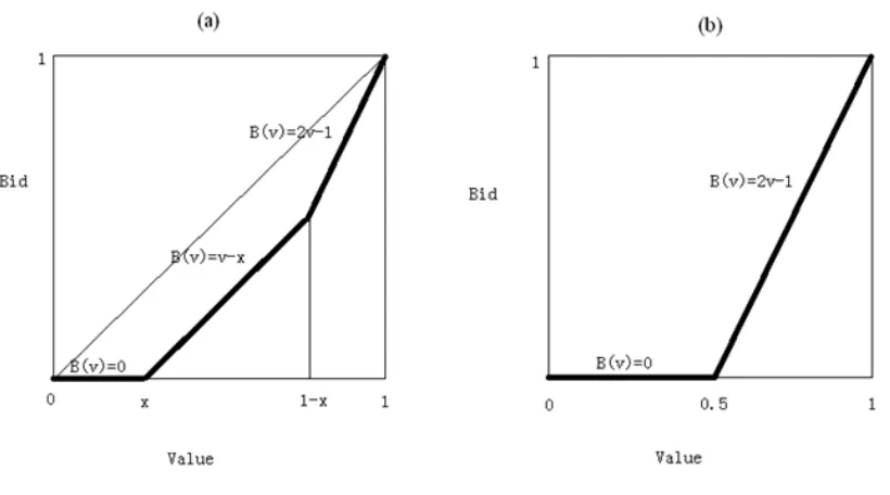
Figure 1: Equilibrium First-Drop Price of R in Clock Auction: (a) 05; (b)≥05
for ∈[121),
() =
⎧ ⎨ ⎩
2
−2
2 , for ∈[01−) 1
2 −, for ∈[1−12]
() =
⎧ ⎨ ⎩
0, when ∈[012] 2−1, when∈(121]
When one bidder has already dropped out, R with value will stay until the clock price
=
⎧ ⎨ ⎩
, if the other remaining bidder is R
min{1 +}, if the other remaining bidder is E .
The entrant stays till =.
Proof. See Appendix.
The equilibrium strategy of a regular bidder when all three bidders are active is shown in Figure 1.
Clearly, regardless of the magnitude of the externality ( is small or large), () for∈(01).
Thus the equilibrium exhibits “free riding” in the sense that the lowest valued incumbent will drop out
of the clock auction before the price reaches his or her value (and both may attempt to drop out at
zero price). The complete proof of Proposition 1 is quite tedious, but the intuition is simple: instead
would be better offby free riding on the other incumbent if the other incumbent has a better chance of beating the entrant. More precisely, this free-riding feature is caused by the combination of the
negative externality and the dynamic nature of the clock auction: without the dynamic nature of the
clock auction, the incumbents simply cannot free ride, as will become clear below, where we develop
the equilibrium for the FPSB auction with the negative externality.
Also note that() is strictly decreasing in, so the endogenous tie-breaking rule (the augmented auction) is efficient in the sense that it will always select the incumbent with the higher value to stay, which improves overall efficiency in the auction.
2.2
The First-Price Sealed-Bid Auction
Again we will characterize the symmetric equilibrium ((·), (·)) where (·) is the equilibrium bid function for the two incumbents and (·) is the equilibrium bid function for the entrant.
Given that the other two bidders follow the proposed equilibrium strategies, incumbent 1bids to maximize his expected payoff:
Π1 = (−1())(−1())(1−)−
Z 1
−1()
Z −1((
))
0
(2)()2
= −1()−1()(1−)−
Z 1
−1()
Z −1
(())
0
2
That (·) is a best response to ((·), (·)) implies Π1 = 0 when evaluated at = (1). This leads to the following equation:
0−1((1))−1((1))(1−(1)) +
0−1
((1))(1−(1))1
−−1((1))1+
0−1
((1))1 = 0
Similarly, the entrant bids to maximize his expected profit:
Π = ((−1()))2(−) = (−1())2( −)
That(·)is a best response to(·) impliesΠ= 0when evaluated at=()or−1() =.
This leads to the following equation:
20−1(())·( −())−−1(()) = 0
In equilibrium the following differential equations should hold simultaneously:
⎧ ⎨ ⎩
0−1()−1()(1−) +
0−1
()(1−)1−−1()1+
0−1
()1= 0
20−1()( −)−−1() = 0
where=(1) and =().
Proposition 2 Under thefirst-price sealed-bid auction (FPSB), the symmetric equilibrium is
character-ized by the differential equations (1) and the boundary conditions(0) =(0) = 0, and(1) =(1) =
for some ∈(01). For ∈(01), () (), i.e., incumbents bid more aggressively than the entrant in equilibrium.
Proof. See Appendix.
Let the inverse bid functions be (·) =−1(·) and(·) =−1(·). Equations (1) can be rewritten
as follows.
⎧ ⎨ ⎩
0()()(()−) +()0()(()−)−()() +0()() = 0 20()(()−)−() = 0
(2)
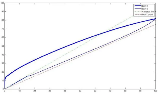
Figure 2 plots the schedules(·)and(·)(based on= 07), along with the equilibrium bid function for a 3-bidder FPSB auction with no externality (given by () = 23).6 As shown(·) lies above(·),
as incumbents bid more aggressively than the entrant in order to avoid the externality. Moreover, the
entrant’s bid function lies above () = 23, as the aggressive bidding of the incumbents heats up the
competition, which in turn requires more aggressive bidding on the part of Es, more aggressive than
under the risk-neutral Nash equilibrium absent an externality. From the figure, it is also clear that
incumbents bid above their values when their values are below some threshold.
In what follows we will be comparing the FPSB and English auctions with respect to revenue,
efficiency, and the probability that an entrant will win the auction.7 Under the assumption of risk neu-trality, revenue differences between the two auction formats increase monotonically with increases in the negative externality, with substantially higher variance in revenue in the English auctions throughout.
With respect to efficiency as measured by the probability with which the bidder with the highest value 6Plotting (
·) forward starting at = 0 is infeasible as 0(0) cannot be determined. So we plot the (numerical)
equilibrium bid schedules backward starting at = 1. ¯ is determined such that (0)and (0)are sufficiently close to
zero. That= 07is chosen as it is consistent with the parameter value used in our experiments.
7The results reported here are based on large sample simulations as there is no closed-form solution for the FPSB
auction. These results will not necessarily hold for smaller sample sizes like those employed in the experimental sessions.
As such, in comparing revenue, efficiency, and frequency that Es win the auction, we also report predicted outcomes based
on the experimental valuations drawn. The most sensitive element with respect to small sample properties has to do
with differences in average revenue. Differences in revenue variance never overlap for the sample sizes employed, with the
Figure 2: Equilibrium Schedules(·),(·), and (·) under FPSA (= 07)
wins the item (where value includes the externality for Rs), the English auction is always efficient. This follows from the fact that there will always be at least one R competing with the entrant, and this R will
remain active up to her value plus the externality. Note however that this efficiency measure ignores the potential implications of entry for increased competition and increased efficiency in the product market after entry. Finally, the probability with which Es win the auction is smaller through out, as E’s value
must be above any R’s value (including the negative externality) in order to win, whereas this is not
the case in the FPSB auctions.
3
Experimental Design
Each experimental session consists offive auctions operating simultaneously with three bidders in each
auction. There are three sessions each for the clock and FPSB auctions with externalities and two
sessions for the FPSB with no externality (a control treatment). Instructions were read out loud with
subjects having copies to follow.8 Each session started with 3 dry runs followed by 25 paid periods. All subjects were paid their end of experiment cash balance. Table 1 shows the number of sessions along
with the number of subjects under each auction format. Each session lasted for approximately one and
a half hours.
Table 1: Experimental Treatments
Session TotalNumber of subjects
Number of
E subjects
Number of
R subjects
Number of
groups
Number of
periods
Clock
CL1 15 5 10 5 25
CL2 15 5 10 5 25
CL3 15 5 10 5 25
FPSB
FP1 15 5 10 5 25
FP2 15 5 10 5 25
FP3 15 5 10 5 25
FPSB Ctrl
FPC1 15 0 15 5 25
FPC1 15 0 15 5 25
Private values for all bidders were drawn iid from a uniform distribution with support [0, 100]
(with integer values only), with new values drawn before each auction. The externality was set at−70
throughout. At the beginning of a session subjects were randomly assigned to be either an E or an R
(referred to as a type A and type B bidder, respectively), and remained in that role throughout. In each
auction subjects were randomly assigned to a new three-bidder market, with each market containing
one E and two Rs.
The clock auction employed a digital price clock starting at 0 and counting up by 2 every second.
The computer screen showed a bidder’s private value, the bidder’s type, the current price of the item,
and the type(s) of other active bidders. Drop-out prices and dropped bidders’ types were reported as
they occurred. Before the start of the auction each bidder had the opportunity to drop out at 0 or to
bid in the auction. If more than one bidder chose to drop at zero, a SPSB auction was conducted to
decide the right to drop out at 0.9 The auction stopped as soon as there was only one active bidder. This last bidder obtained the item and paid the price at which the next-to-last bidder dropped out. At
the end of the auction, the price paid for the item and the winner’s type were announced to all bidders,
with earnings reported privately to each bidder. A complete history of these outcomes was available to
each bidder as well.10
In the FPSB auction, each bidder entered an integer bid. The bidder with the highest bid obtained
the item and paid a price equal to his bid. In the case of ties the computer randomly determined who
got the item. Losing bidders each incurred a loss of 70 if E won, and zero profit if an R won. Subjects
were permitted to bid above their valuations, with incumbents permitted to bid above their valuations
plus the externality, although both of these outcomes were rarely observed.
At the beginning of each session, Es were given an initial cash balance of 500 experimental currency
units (ECUs) with Rs having a starting balance of 900 ECUs. The difference in initial cash balance was calibrated to account for losses due to the externality, and for expected differences in auction earnings between player types. These starting cash balances were private information so that Es would not have
been aware of the larger starting cash balances for Rs. Cash balances were 500 ECUs in the FPSB
control sessions. Subjects were paid their end of session balances in cash with ECUs converted into
Chinese yuan at the rate of 10 ECUs = 1 yuan. Earnings averaged 72 (45) yuan for Rs and 52 (54)
yuan for Es in the clock (sealed-bid) auctions. Under the prevailing exchange rate this averages out to
about $9 US dollars per subject.11 Starting cash balances were sufficient to insure zero bankruptcies.
All subjects had no previous experience with any type of auction experiment, although some of them
may have had experience in another experiment.
An explicit control treatment was employed for the FPSB auction since subjects are known to bid
well above the risk-neutral Nash equilibrium in the absence of a negative externality (see, for example,
the many references cited in Kagel, 1995). As such a control treatment is needed to compare bidding
with and without the externality. In contrast, bidding in English clock auctions absent externalities
are known to converge to the dominant bidding strategy. This is confirmed here by bids in the clock
auction when only two regular bidders remained active. The size of the externality employed was quite
large as earlier experimental results under a similar design with a much smaller negative externality
had a very limited impact on subject behavior, and provided little scope for learning.12
1 0The software was programmed using zTree (Fischbacher, 2007).
1 1
This is a little higher than the average student wage which, for local college students with a standard work load which
averages between 10 and 20 yuan per hour. (The clock auctions averaged 2 hours, with the sealed bid auctions lasting
about 1.5 hours.)
1 2See Hu et al. (2010) for these results. This experimental design used a random tie-breaking rule in case two or more
bidders dropped out at the same time prior to the start of the auction. This does not result in a well defined equilibrium
Subjects were recruited through posters from among the undergraduate students from various
de-partments at Southwestern University of Finance and Economics in Chengdu, Sichuan Province, China.
In 2011, Southwestern ranked 32 overall in China for undergraduate education, ranking 30th for
Fresh-men quality based on Chinese college entrance exam scores.
4
Experimental Results
4.1
Bidding in Clock Auctions
In the analysis that follows, unless stated otherwise, data will be reported for the last 12 auctions in each
experimental session, after subjects have had some experience with the auction contingencies. Results
are similar to those for the entire set of auctions, but somewhat closer to equilibrium outcomes, as
there is some learning. Results for the entire set of auctions are reported in the online appendix to the
paper.13
In what follows we report the experimental results in the form of a number of conclusions followed
by the data supporting those conclusions.
Result 1 In terms offirst drop outs, there is substantial, but far from complete free riding on the part of
Regular bidders (Rs) as the theory predicts.
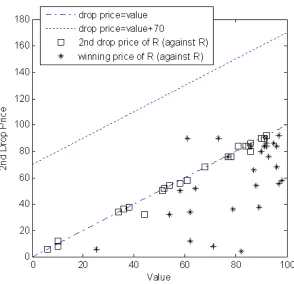
Figures 3 and 4 shows thefirst drop price against values in the clock auctions for Rs and Es separately,
along with the equilibrium bid functions.14 There is a mass of zero, or close to zero, bids on the part
of Rs with values in the interval [0, 50] as the theory predicts: R’s with values less than or equal to 50
dropped at or before the clock auction started 34.7% of the time.15 There are also a number of drops
at, or close to value (the 45 degree line), representing a failure to free ride, even at low values. Further,
Rs’ stage-one drops along the 45 degree line, although not the free riding the theory predicts, stand in
auctions were rare (5 out of 275 auctions) so the random tie breaking rule had little impact on the outcomes. The size of
the negative externality in this earlier experiment was 20, with values drawn from the support [0, 100].
1 3
http://www.econ.ohio-state.edu/kagel/Externality.
1 4Thisfigure excludes the 10 cases in which a bidder who dropped prior to the start of the auction and lost the SPSB
auction.
1 5In contrast, when an R’s value was greater than 50, he/she dropped out before the clock started less than 2% of the
time. For Es with values less than or equal to 50, the overall frequency of dropping before the clock started was 13.9%.
market contrast to the frequency with which Rs drop with bids above their value (or win the auction
[image:14.612.217.405.135.430.2]with bids above value) when competing with Es after stage-one (see Figure 6 and 7 below).
Figure 3: First Drop Prices for Rs
Result 2 The frequency with which both Rs drop out before the start of the auction is much less than
predicted. The frequency with which the lowest value R wins the right to drop out in the tie-breaking
auction is quite low as well, substantially lower than when neither R drops out, or only one R drops
out, prior to the start of the auction. As a result efficiency is substantially greater in cases where both
bidders fail to drop out prior to the start of the auction.16
There were only 10 SPSB (tie-breaking) auctions in which both Rs had values less than or equal
to 50 and both dropped out prior to the start of the auction, much less than the predicted number of
1 6Given the low frequency with which both Rs dropped out prior to the start of the auction, the data reported on here
Figure 4: First Drop Prices for Es
simultaneous drops, 91.17 In 3 of these 10 cases the SPSB auction achieved the efficient outcome, with
the lower valued R winning the right to not participate in the auction.18 In equilibrium in the SPSB auction bids are decreasing in value, so that a lower valued R should submit a higher bid in order to win
the right to drop. But Figure 5 shows that bids in the SPSB do not decrease in value, although most of
the SPSB bids are located below the equilibrium bid function curve. This failure to achieve consistently
high efficiency in SPSB auctions is not surprising given the results from past Vickrey auctions (Kagel, 1995; Kagel and Levin, 2012). In contrast, when both Rs had values less than 50, but only one bidder
dropped out prior to the start of the auction, the lower valued R dropped first 71% of the time; and
when neither bidder dropped out prior to the start of the auction, the lower valued R droppedfirst 62%
1 7
There were 7 cases where an R and E both dropped prior to the start of the auction, and one case in which all three
bidders chose to drop prior to the start of the auction.
1 8
of the time. While the latter is a direct consequence of the fact that many Rs who failed to drop at or
[image:16.612.198.428.132.363.2]near zero tended to bid up to their valuations, the former is not.
Figure 5: Bids in SPSB Auctions
Result 3 In clock auctions with two bidders being active, bids are close to equilibrium levels for Rs
but not Es: Rs tend to drop at their value when the remaining bidder is an R, and at their value plus
the externality (70) when the remaining bidder is an E. While a number of Es followed the dominant
strategy, a considerable number consistently bid above their values.
Figures 6 and 7 show, respectively, drop outs and winning bids for those sub-auctions where the
remaining bidders were an E and an R. Two factors stand out. First, there are a large number of
instances in which Es, contrary to the dominant bidding strategy, dropped out with bids above their
values (68.7% of all Es dropping out second), but only a handful of auctions where Es wound up with
a winning bid above their value (6.0% of these sub-auctions).19 Second, there were large numbers of
1 9Amending these calculations to allow for rounding error, or momentarily being distracted as the clock ticked up, to
bidding above value + 4 ECUs, these percentages become 58.2% and 4.6%, respectively. Es won 17 auctions in total, with
losses in 9 of the auctions. In 7 of these 9 auctions, Rs dropped out prior to bidding up to their value plus the externality.
auctions in which Rs won with bids above their value (but less than the externality; 53.6% of these
sub-auctions). There was some heterogeneity in the extent to which Es consistently bid in excess of
their value, with 60.0% of Es bidding above their value more than 50% of the time.20 In contrast, 100%
[image:17.612.161.464.173.407.2]of Rs either won or bid up to their value plus the externality more than 50% of the time.
Figure 6: Stage-Two Bids in Clock Auctions: Both R and E Active
Figure 8 reports dropouts and winning bids for those sub-auctions where both bidders were Rs. In
this case Rs’ behavior is generally consistent with the dominant strategy as drop out prices hover around
the 45 degree line, and there were only two auctions in which Rs won with bids above their value when
competing against another R.21
We were, quite frankly, surprised by the high frequency of Es bidding above their value. However,
there is precedence for this in the literature: Andreoni, Che, and Kim (2007) report a series of SPSB
private value auctions under varying information about rivals values. Most relevant to our experiment is
their 1 x 4 auctions in which all four bidders had full information about each others values, which they
2 0This includes winning bids above value.
2 1Dropped from Figure 8 are those sub-auctions in which when E dropped both Rs were still active with one or both
bidding above their value. There is an obvious incentive in these cases for Rs bidding above value to drop immediately,
Figure 7: Wining Prices in Clock Auctions: Both R and E Active in Stage 2
compared to their 4 x 1 treatment in which none of the bidders had any information about each others’
values. Absent information about rivals values 85.5% of all bids were sincere (equal to value) versus
62.5% sincere bidding in auctions with full information.22 12.0% were above value without information
and 25.3% above value with full information. That is, with full information about rivals valuations,
there was a sharp increase in bidding above value which can be attributed to spiteful bidding. While Es
in our auctions do not know Rs values, they do know that in sub-auctions in which they are competing
with an R, the R has an incentive to bid up to their value plus the amount of the externality. This
allows Es to engage in spiteful bidding relatively safely as long as their bids stayed at or below 70, and
to do so with added risk for bids above 70. Looking back at Figure 6 this is consistent with the pattern,
as Es bidding above value tapers offa bit for values above 70.23 Finally, note that there are relatively few bids below value in Figure 6, in contrast to the 12.3% of bids below value reported in the Andreoni
2 2
Calculations are over the last 10 auctions out of the 20 conducted. Note, their subjects were undergraduates at the
University of Wisconsin.
2 3
When Es dropped second in these sub-auctions, their frequency of dropping above value plus 4 ECUs was 64.3% for
Figure 8: Stage-Two Bids and Winning Prices in Clock Auctions: Both Rs Active
et al. full information treatment, which is suggestive of greater rivalistic bidding in China compared to
Wisconsin.
4.2
Bidding in FPSB Auctions
Result 4 Consistent with the theory, Rs tend to bid more aggressively (higher) than Es in FPSB
auctions. Also consistent with the theory, Rs and Es tend to bid more aggressively than in the FPSB
independent private value auctions (the control treatment).
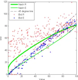
Figure 9 plots bids for Rs and Es in the FPSB auctions, along with the equilibrium bid functions.
The graph shows that Rs bid higher than Es, on average, for all valuations, with Rs’ bids at lower
valuations closer to their value plus the externality than the risk-neutral Nash equilibrium (RNNE).
Figure 10 graphs bids for Rs compared to the controls, with Rs bidding higher than the controls, on
average, at all valuations. Note that 10 shows the standard result for independent private value FPSB
bids of Es compared to the controls. Es tend to bid higher than the controls, particularly at higher
valuations. This occurs in spite of the rather massive overbidding relative to the RNNE in the controls.
Finally, there is minimal bidding above value for Es and the controls, with no bids above their value
[image:20.612.175.447.177.456.2]plus the externality for Rs.24
Figure 9: Bids in FPSB Auctions with Externality Present
Random effect regressions, with subject as the random component, reported in Table 2 confirm these results. In these regressions we have dropped bids for valuations less than 10 as (i) the equilibrium bid
function with externalities has its most pronounced non-linear component in the interval [0, 10], and (ii)
at low valuations there is some tendency for “throw away” bids as subjects realize they have very little
chance of winning the auction with very low valuations. Several specifications are reported, with and
without a 2 term. All of the specifications treat the controls as the reference point against which to
compare Rs and Es bids. There is a separate dummy variable with value 1 if the subject is an R, and 0
Figure 10: Bids in FPSB Auctions: Rs versus Controls
otherwise, a separate dummy with value 1 if the subject is an E, and 0 otherwise, and interaction terms
for each of the two dummies and and for the two dummies and the2 term. Although including the
E*2 and the R*2 interaction effects shows that neither of these variables being statistically significant in their own right, and results in the E* interaction term no longer being statistically significant, a
chi-square test shows that we can reject a null hypothesis at the 1% level that (i) the E* interaction
terms and the E*2 interaction terms are jointly equal to zero and (ii) the R* interaction terms and
the R*2 interaction terms are jointly equal to zero as well.
Figure 12 plots the estimated bid functions for Rs, Es and the controls for the right hand most
specification in Table 2, our preferred specification. Evaluating the estimated bid function for this
Figure 11: Bids in FPSB Auctions: Es versus Controls
theory predicts. Similarly, Es were bidding significantly more than the controls ( 005) for higher
valuations ( 53), with the differences between Es and the controls not significantly different from each other for values less than this. Finally Rs were bidding significantly more than Es at lower valuations
( 78), with no significant differences between the two at higher valuations. These results are all qualitatively consistent with the theory since differences in bids between Es and Cs are minimal at lower valuations, with differences in bids between Rs and Es growing smaller at higher valuations. As a side note, the negative sign for the 2 term reflects the fact that at the very highest valuations the
tendency to bid well above the risk-neutral NE in IPV FPSB auctions tends to be moderated (see, for
Table 2: Random Effect Regressions. Dependent Variable: Bids in FPSB Auction
FPSB w/ & w/o Externality
Value10
Period 14-25 14-25 14-25
Constant 1.99*** (0.65)
-1.80
(1.17)
-3.25***
(1.13)
E Dummy -1.74 (1.55)
-1.89
(1.48)
-1.91
(2.63)
R Dummy 33.95*** (3.62)
34.02***
(3.60)
37.73***
(4.70)
Value 0.81*** (0.02)
0.99***
(0.05)
1.06***
(0.05)
E×Value 0.09*** (0.02)
0.09***
(0.02)
0.09
(0.11)
R×Value -0.29*** (0.05)
-0.30***
(0.05)
-0.47***
(0.14)
Value2 - -0.0016***
(0.0005)
-0.0022***
(0.0005)
E×Value2 - - 0.000017
(0.000923)
R×Value2 - - 0.0016
(0.0012)
Obs 802 802 802
R-sqrd 0.85 0.85 0.85
Standard deviations in parenthesis. ***Significant at 1 percent level,
two tailed test; **Significant at 5 percent level, two tailed test; * Significant
Figure 12: Estimated Bid Functions for FPSB Auctions: v10, including Vsq.
4.3
Revenue and E
ffi
ciency
25Result 5 The FPSB auctions have higher average revenue and smaller variance in revenue than the
clock auctions. The former is not statistically significant at conventional levels, but the latter is.
Table 3 compares average revenue under the two auction formats where predicted revenue is based
2 5Statistical tests throughout this section are based on OLS regressions in which the dependent variable consists of session
average values for the variable in question and right hand side variables consist of dummy variables for the treatment
conditions. For example, with revenue as the dependent variable, right hand side variables consist of a dummy variable
for FPSB auctions with the negative externality = 1 (0 otherwise) and a dummy for the FPSB control auctions = 1 (0
otherwise), with the omitted treatment (English clock auctions) represented by the constant. Use of session value averages
for the dependent variable represents the very conservative assumption that each auction session is a single observation
because of complete autocorrelation of observations due to random re-mixing of subjects between auctions (see Frechette,
2012, for a discussion of statistical issues involved in, and alternative ways of dealing with, the typical practice of re-mixing
subjects between rounds in experiments). Given the clear theoretical predictions regarding efficiency and entry rates
on auction valuations used in the experiment. Predicted revenue is higher under the FPSB auction
than under the clock auction. Actual revenue is substantially higher than predicted revenue in the
FPSB auctions, which is not unexpected given the overbidding (relative to the RNNE) typically found
in FPSB auctions without externalities. Actual revenue is substantially higher than predicted revenue
in the clock auctions as well. This is a result of Es bidding above value. Revenue is higher in the FPSB
auctions than in the clock auctions, but this difference is not statistically significant at conventional levels, largely on account of bidding above value on the part of Es.26
Absent a negative externality, and assuming risk neutral bidders, the variance in revenue in English
auctions is predicted to be greater than in the FPSB auctions. With the negative externality this
tendency is exaggerated as the remaining incumbent bidder is willing to bid up to his value to forestall
entry, with the entrant bidding up to his value. This prediction is indeed satisfied in our experiment
with the variance in revenue in the English auctions substantially higher than in the FPSB auctions
(743.6 versus 130.7; p0.01).
Finally, as expected, average revenue is significantly higher in both the clock auctions and the FPSB
auctions with the negative externality than in the FPSB no externality auctions (p 0.01 in both
[image:25.612.118.516.427.597.2]cases).
Table 3: Revenue, Efficiency and Percent of Auctions E Win
Ascending clock FPSB Difference
Actual Predicted Actual Predicted Actual Predicted
Revenue 73.00
(2.03)
63.69
(2.12)
75.99
(0.87)
67.92
(0.84)
2.99 4.23
Efficiency 76.67
(3.16)
100.00
(0.00)
66.11
(3.54)
85.56
(2.63)
-10.56*** -14.44
% E Win 9.44
(2.19)
0.56
(0.56)
20.00
(2.99)
17.78
(2.86)
10.56* 17.22
Notes: Standard deviation in parenthesis.
* Significant at the 0.10 level. *** Significant at the 0.01 level.
2 6
Es overbidding is present to begin with but grows substantially in frequency over time (36.4% of all Es bids in thefirst
13 auctions vs 58.3% in the last 12). As a result revenue is significantly higher in the FPSB auctions than in the clock
Result 6 The clock auctions are significantly more efficient than the FPSB auctions when the
exter-nality is present, and the FPSB control auctions are significantly more efficient than both auctions with
the externality present.
We measure efficiency strictly in terms of the frequency with which the highest valued bidder wins the auction. In calculating this, Rs value include the cost of the externality as well as their private
value. In equilibrium the clock auction is predicted to be 100% efficient because free riding only exists in thefirst-stage of the auction, with bidders having a dominant strategy to bid up to their valuations
after that. In contrast, the FPSB auction with the externality is akin to an auction with asymmetric
valuations, so that efficiency will, in general, be less than100%.
Table 3 reports average predicted and actual efficiency in the two auction formats with the externality present, where predicted efficiency is for the auction valuations actually drawn. Actual efficiency is significantly lower in the FPSB auctions than in the clock auctions, with the difference reasonably close to the predicted difference, in spite of the fact that absolute efficiency values are well below predicted levels in both cases. Note that the efficiency measure here excludes any potential increase in efficiency for the market in question given the predicted increase in entry fro the FPSB versus the English auctions.
A more complete measure of efficiency would take this effect into account.
Finally, the asymmetric nature of the FPSB auctions with the externality results in substantially
lower efficiency compared to the FPSB control auctions (66.1% vs 88.3%, p0.01). The FPSB control auctions are significantly more efficient than the clock auctions as well (p0.05).
Result 7 Es win more often in the FPSB auctions than in the clock auctions.
Table 3 reports the proportion of auctions won by Es. Es are predicted to win substantially more
often with the FPSB auctions compared to the clock auctions, with this result just failing to achieve
statistical significance at the 10% level (p = 0.052). Given the weak power of this test due to the
limited number of experimental sessions, it is worthwhile noting that using session averages based on all
the auctions within a given experimental condition, entry is significantly greater in the English auctions
at better than the 5% level. Thus, to the extent one can draw policy implications from the present
experiment, our results indicate that if policy makers want to encourage entry they should adopt the
5
Conclusion
This paper investigates theoretically and experimentally the effect of a negative externality on bidding strategies in an English clock auction and afirst-price sealed-bid auction with two incumbents and one
potential entrant. On the theoretical front, the equilibrium analysis shows that in the English auction
one of the incumbents will typically engage in severe free riding. When this happens, the remaining
incumbent bids quite aggressively to deter entry, bidding up to his value plus the potential cost of the
negative externality. In the first-price sealed-bid auction, free riding and aggressive bidding coexist
for incumbents as there is no way for bidders to implicitly coordinate their actions as in the English
auction, resulting in incumbents bidding more aggressively than the potential entrant in order to avoid
the externality. This in turn induces the entrant to bid more aggressively than in an auction with no
externality present.
We observe substantial, though far from complete free riding in the clock auction treatment. Further,
in those sub-auctions where the remaining incumbent competes against the entrant, incumbents bid
reasonably close to the equilibrium level predicted, well above their private value in order to deter the
entrant. While bids are close to equilibrium levels for regulars they are not for entrants, with many
of the latter bidding well above their valuations. Looking at the extant literature suggests that this
is not some odd behavior of our sample population. But rather it reflects rivalistic bidding of the sort
found in Andreoni et al. (2007) in second-price sealed-bid auctions when all bidders’ valuations are
common knowledge. Bidding in the first-price auctions, while well above the levels predicted under the
risk-neutral Nash equilibrium, tends to satisfy the qualitative predictions of the equilibrium with regular
bidders bidding higher than entrants, and both regular bidders and entrants bidding higher than in a
first-price auction with no externality present. Qualitative predictions regarding higher revenue and
lower efficiency in the sealed-bid versus clock auctions, along with the likelihood of the entrant winning the auction, are satisfied in the data as well.
Our model follows the literature using the term “externality” to measure the negative payoff to an incumbent when losing the auction. Perhaps a more proper term might be “post-auction effects.” Extensions can be made to enrich the post-auction interactions, so that the “externality” would be a
variable endogenously determined by the post-auction game. Investigation of this issue is left for future
Appendix
Proof of Proposition 1
Derivation of (·)
It is obvious that remaining active until the price reaches his value is a (weakly) dominant strategy for
the entrant (E). It is also clear that the equilibrium bidding strategies after one bidder has dropped out
should be the ones specified in the proposition.
We will first derive the form of (·) using the necessary equilibrium conditions (we will verify the sufficiency later). Suppose that incumbent 1 (R1) drops at(ˆ1) while incumbent 2 (R2) follows(·), where ˆ1 is sufficiently close to 1. Clearly, R1 cannot benefit from dropping higher than (1) when the other two bidders are still active. So we only need to consider ˆ11. Let ∆(1ˆ1) be the change in R1’s expected payoffs (from dropping at (ˆ1) instead of (1)). We first discuss the case where
12.
1. 1∈[1−1). If he deviates upwards, his payoffchanges only when2 ∈(1ˆ1)and (2). If he deviates downwards, it only affects his payoff when he prevents another bidder (R2 or E) from dropping between(1)and (ˆ1). Hence,
∆(1ˆ1) =
⎧ ⎪ ⎪ ⎪ ⎨ ⎪ ⎪ ⎪ ⎩
Z ˆ1
1
Z 1
(2)
(1−)2, when ˆ1 1
Z 1
ˆ
1
Z 1
(2)
(−1)2+
Z (1)
(ˆ1)
Z 1
−1(
)
(2−1)2, when ˆ1 1
For (·) to constitute a symmetric equilibrium, we must have the followingfirst-order conditions:
lim
ˆ
1→+1
∆(1ˆ1)
ˆ1
= 1
2[1−(1)]·[21−1−(1)] = 0
lim
ˆ
1→1−
∆(1ˆ1)
ˆ1
= 1
2[1−(1)]·[−21+ 1 +(1)] = 0
Thus we must have (1) = 21−1 for1∈ [1−1).
2. 1∈ [1−), where is the minimum value for an incumbent to drop above price zero. In other words,is the (equilibrium) cutoffvalue under which an incumbent will drop out at the beginning of the clock auction (when the price equals 0). We do not impose any constraint on for the
If he deviates upwards and the dropped bidder happens to be R2, we have 2 ∈ (1ˆ1), and
the identities of the two remaining bidders will change from R2 and E to R1 and E and the
deviation payoffs can be obtained accordingly; if the dropped bidder happens to be E, we have
∈((1) (ˆ1)), and the identities of the two remaining bidders will change from R2 and E to R2 and R1. If she deviates downward, the situations can be analogously examined. Taking all
together, we have
∆(1ˆ1) =
⎧ ⎪ ⎪ ⎪ ⎪ ⎪ ⎪ ⎪ ⎨ ⎪ ⎪ ⎪ ⎪ ⎪ ⎪ ⎪ ⎩
Z ˆ1
1
Z 2+
1+
(−)2+
Z ˆ1
1
Z 1+
(2)
(1−)2, when ˆ1 1
Z 1
ˆ
1
Z 1+
2+
(−−1+)2+
Z 1
ˆ
1
Z 2+
(2)
( −1)2
+
Z (1)
(ˆ1)
Z 1
−1(
)
(2−1)2, when ˆ1 1
For (·) to constitute an equilibrium, we must have
lim
ˆ
1→1+
∆(1ˆ1)
ˆ1
= 1 2
n
[1−(1)]2−2
o
= 0
lim
ˆ
1→−1
∆(1ˆ1)
ˆ1
= 1
2[1+−(1)]·[−1++(1)] = 0
Since (1) =1+ cannot be the equilibrium strategy, we must have(1) =1− for1 ∈
[1−), which also implies that =.
For the case≥12, the analysis is essentially the same except that there is a change in the supports
of the piecewise function(): the second segment now vanishes because≥1−. The lower bound of the second segment should now be 12 instead of1−due to the continuity of (), which implies
that the incumbent with= 12 should be indifferent.
Note that()so derived is unique. This means that should a symmetric equilibrium strategy exist, it must be uniquely determined for≥. It’s also worth noting that the uniqueness and the functional
form of(·) are independent of the tie breaking rule at = 0.
Derivation of (·)
Let () be the expected contingent payoff for an incumbent with value who loses the augmented auction. We have
() =
Z min{1+}
0
(−) +
Z 1
min{1+}
(−) = ⎧ ⎨ ⎩
(+)2
2 −, for≤1−
Suppose() is strictly decreasing in . R1 with value1 bids(ˆ1) to maximize
(ˆ1 1) =
⎧ ⎨ ⎩
Rˆ1
0 (1)2+
R
ˆ
1
h
−(2) +Rmin1 {12+}(−)
i
2, for 12
2Rˆ1
0 (1)2+ 2
R1 2
ˆ
1
h
−(2) +Rmin1 {12+}(−)
i
2, for≥ 1 2
(3)
For (·) to constitute a symmetric equilibrium, we must have (ˆ1 1)ˆ1|ˆ1=1 = 0, which
leads to, when 12,
() =
2−2
2 , for∈[0 ]
and when ≥ 12,
() =
⎧ ⎨ ⎩
2
−2
2 , for∈[01−) 1
2 −, for∈[1−12]
For consistency check, () so derived is indeed decreasing in. Also note that () = 0 at=
when 12and at = 12 when ≥12.27 Substituting the expressions of () into (3) and then differentiating(ˆ1 1) with respect toˆ1, we have
½
(ˆ1 1)
ˆ1
¾
=
⎧ ⎨ ⎩
n(1−ˆ1)
³
1+ˆ1
2 +
´o
, for 1−
{1−ˆ1}, for≥1−
which is positive when ˆ1 ≤ 1 and negative when ˆ1 ≥ 1. This shows that () given above is the unique symmetric equilibrium bid function in the augmented auction.
Therefore, if both incumbents are to drop at zero when their values are both belowwhen 12
and below 12when ≥12, then in the augmented auction no party has an incentive to deviate from
bidding(·) should the other follow(·).
Verification of Equilibrium (·)
We will consider incumbent 1 (R1) whose value is1. Given that the other incumbent (R2) follows(·) and the entrant (E) stays till the price reaches his value, we will evaluate the change in his expected
payoffby deviating to drop at (1±) instead of (1), where 0 and1±∈[0min{1+1}]. Dropping at a price higher than 1+ or1 is obviously a dominated strategy. We willfirst examine
the upward deviation, followed by the downward deviation.
We consider the case 12first.
2 7It is easily seen that an incumbent with=when 12and= 12when
≥12is indifferent between dropping
out at zero and staying (but droping out immediately after the clock starts). For incumbents who are not suppposed to
1. Upward deviation. R1’s deviation will affect the auction outcome only when it allows another bidder to dropfirst at ∈((1) (1+)). We discuss three sub-cases in order:
1.1. 1 ∈[0 ]. R1 is supposed to drop at = 0. We will consider two possibilities for 2: 2 ∈[0 ] and 2∈(1]and show that it is not profitable for R1 to deviate regardless of the value of2.
1.1.a. 2 ∈ [0 ]. R2 drops at zero in equilibrium. If 2 1, both the tie breaking rule and the deviation to(1+)0will make R1 stay with E, and the auction outcome will stay the same.
If2 ≥1, we already show that there is no incentive to deviate from(·)conditional on dropping out, so we only need to rule out the possibility of dropping at a price strictly above zero. The
auction outcome will be different if either of the two events occurs: the outcome changes from R2 winning against E to E winning against R1 or from R2 winning against E to R1 winning against
E. Note that by this deviation, R1 can avoid paying (2), which is his equilibrium payment in the augmented auction. The change in R1’s expected payoffis given by
Z
1
Z 2+
1+
(−)2+
Z
1
Z 1+
0
(1−)2+
Z
1
(2)2
= −1
3(−1)(2
2−
1−21)≤0
Therefore the deviation will make R1 worse offif2∈[0 ].
1.1.b. 2 ∈(1]. When the current price is 0, R1’s deviation to dropping at (1+)(0) instead of
0 will affect the outcome only when it allows another bidder to drop first at ∈(0 (1+)). There are two possible cases: 1+∈(1−]and1+∈(1−1].
When 1+∈(1−], if R2 drops first after the deviation, it implies that2 ∈( 1+) and
∈(2−1]. The two remaining bidders will change from R2 and E to R1 and E. The auction outcome could be affected in either of the two events: the outcome changes from R2 winning against E to E winning against R1; or from R2 winning against E to R1 winning against E. If
instead E drops first after the deviation, we have that ∈(0 1+−) and 2 ∈ ( +1].
The two remaining bidders will change from R2 and E to R2 and R1. R2 will win in both cases;
thus R1’s payoffwill be zero. To sum up, the change in R1’s expected payoffis given by
Z 1+
Z 2+
1+
(−)2+
Z 1+
Z 1+
2−
(1−)2
= 1 2
Z 1+
Since 2 ∈[1 1+] and ≤, we have 1 ≤2 and 1−2 ≥ −. Therefore R1 will be worse
off from the deviation. When 1+ ∈ (1−1], the argument is similar as above except that
22−1 is R2’s bid function when 2 ∈(1− 1+). It can be demonstrated analogously that
the change in R1’s expected payoffis also negative.
1.2. 1 ∈(1−). We will consider two possible cases: 1+∈(11−) and 1+∈[1−1). (1+= 1is not possible because of the restrictions that 1 1− and ≤.)
1.2.a. 1+ ∈ (11−). If R2 drops first after the deviation, it implies that 2 ∈ (1 1 +) and
∈(2−1]. The identities of the two remaining bidders will change from R2 and E to R1 and E. Such a deviation can change the outcome in two possible events: the outcome changes from
R2 winning against E to R1 winning against E, and R1’s payoffchanges from 0 to1−; from
R2 winning against E to E winning against R1, and R1’s payoffchanges from0to−. If E drops
first after the deviation, it implies that ∈(0 1+−) and2 ∈(+1], and the identities
of the two remaining bidders will change from E and R2 to R1 and R2. The fact that R2 is active
when the price has reached(1) implies that 2≥1. R2 will win in both cases and R1’s payoff is not affected by the deviation. Therefore, The change in R1’s expected payoffis given by
Z 1+
1
Z 1+
2−
(1−)2+
Z 1+
1
Z 2+
1+
(−)2
= 1 2
Z 1+
1
(1−2)·(1−2+ 4)2
which is negative for the same reason as above. Therefore R1 will be worse off from the deviation.
1.2.b. 1+∈[1−1). If R2 drops first after the deviation, it implies that either2 ∈(11−) and
∈(2−1], or2 ∈[1− 1+)and ∈(22−11]. The identities of the two remaining
bidders will change from R2 and E to R1 and E. Such a deviation can change the outcome in two
possible ways: the outcome changes from R2 winning against E to R1 winning against E, and R1’s
payoffchanges from 0 to1−; from R2 winning against E to E winning against R1, and R1’s
payoff changes from 0 to −. If bidder E drops first after the deviation, it implies that either
∈ (01−2) and 2 ∈ ( +1], or ∈ [1−22(1 +)−1) and 2 ∈ (2+11]. The
identities of the two remaining bidders will change from E and R2 to R1 and R2. The fact that
R1’s payoffs will both be zero. Combining these two cases, the change in R1’s expected payoffis given by
Z 1−
1
Z 1+
2−
(1−)2+
Z 1−
1
Z 2+
1+
(−)2+
Z 1+
1−
Z 1+
22−1
(1−)2+
Z 1+
1−
Z 1
1+
(−)2
= 1 2
Z 1−
1
(1−2)·(1−2+ 4)2+
Z 1+
1−
(1+−1)2
+1 2
Z 1+
1−
£
12−2+ (21−22+ 1)·(1−22)¤2
which is negative for the same reason as above. Therefore R1 will be worse offfrom the deviation.
1.3. 1 ∈ [1−1). If R2 drops first after the deviation, it implies that 2 ∈ (1 1 +) and ∈
(22 −11]. The identities of the two remaining bidders will change from R2 and E to R1 and E. Such a deviation will change the auction outcome from R2 winning against E to R1 winning
against E, and R1’s payoffchanges from0to1−. If E dropsfirst after the deviation, it implies
that ∈(21−12(1+)−1)and 2 ∈(2+11]. The identities of the two remaining bidders
will change from E and R2 to R1 and R2. R2 will win in both cases and R1’s payoffs will both be zero. The change in R1’s expected payoffis thus given by
Z 1+
1
Z 1
22−1
(1−)2= 2
Z 1+
1
(1−2)(1−2)2
which is non-positive because 1≤2 and 2≤1. Therefore when 1 ∈[1−1), R1 will not be
better offfrom an upward deviation.
We have thus shown that for all 1 ∈ [01], incumbent 1 will not be better off from any upward deviation.
2. Downward deviation. Incumbent 1’s deviation will affect the auction outcome only when it pre-vents another bidder from droppingfirst at ∈((1−) (1)). We only need to consider two
possible cases: 1∈(1−]and 1 ∈(1−1], as we have proved that conditional on dropping out, incumbents with values less than will follow(·).
2.1. 1∈(1−]. We willfirst consider the deviation of dropping at(1−) = 0, and then consider
2.1.a. 1−≤. Let(1ˆ1)be the deviation payofffor R1by mimicking typeˆ1. We have(1 1)
( ). If 2 ≤ , there is no profitable downward deviation to dropping at zero, as type does not have an incentive to deviate downward, and that type1 and type receive exactly the
same payoffwhen deviating downward. If 2 , the deviation will affect the outcome only if it prevents R2 or E from droppingfirst at ∈[0 (1)). If R2 is the one being prevented, we have
2∈( 1) and ∈(2−1]. The identities of the remaining bidders will change from R1 and E to R2 and E. The auction outcome can be affected in two ways: the outcome changes from R1 winning against E to E winning against R2 or from R1 winning against E to R2 winning against
E. If bidder E is prevented from droppingfirst, it implies that ∈[0 1−) and2∈(+1].
The identities of the remaining bidders will change from R1 and R2 to E and R2. The outcome
can be affected in two ways: the outcome changes from R1 winning against R2 to R2 winning against E or from R2 winning against R1 to R2 winning against E. Given all these, the change in
R1’s expected payoffis given by
Z 1
Z 1+
2+
(−−1+)2+
Z 1
Z 2+
2−
(−1)2+
Z 1−
0
Z 1
+
(2−1)2
= −1 2
Z 1
(1−2)·(1−2+4)2−
1 2
Z 1−
0
(−1++)2
which is negative since 2 ≤1. Therefore R1 will be worse offfrom the deviation.
2.1.b. (1−)∈(0 (1)). If R2 is prevented from droppingfirst, it implies that 2 ∈(1− 1)and
∈(2−1]. The identities of the remaining bidders will change from R1 and E to R2 and E. The auction outcome can be altered in two ways: the outcome changes from R1 winning against E
to E winning against R2 or from R1 winning against E to R2 winning against E. If E is prevented
from droppingfirst, it implies that ∈(1−− 1−) and 2 ∈( +1]. The identities
of the remaining bidders will change from R1 and R2 to E and R2. The auction outcome can be
altered in two ways: the outcome changes from R1 winning against R2 to R2 winning against E or
from R2 winning against R1 to R2 winning against E, and R1’s payoffis not affected. Therefore, the change in R1’s expected payoffis given by
Z 1
1−
Z 1+
2+
(−−1+)2+
Z 1
1−
Z 2+
2−
(−1)2+
Z 1−
1−−
Z 1
+
(2−1)2
= −1 2
Z 1
1−
(1−2)·(1−2+4)2−
1 2
Z 1−
1−−
(−1++)2