Interactive Fuzzy Programming for Random Fuzzy
Two-Level Integer Programming Problems through
Fractile Criteria with Possibility
Masatoshi Sakawa, Takeshi Matsui
Department of System Cybernetics, Graduate School of Engineering, Hiroshima University, Higashi-Hiroshima, Japan Email: [email protected], [email protected]
Received April 17, 2013; revised May 17, 2013; accepted May 24, 2013
Copyright © 2013 Masatoshi Sakawa, Takeshi Matsui. This is an open access article distributed under the Creative Commons Attri-bution License, which permits unrestricted use, distriAttri-bution, and reproduction in any medium, provided the original work is properly cited.
ABSTRACT
This paper considers two-level integer programming problems involving random fuzzy variables with cooperative be- havior of the decision makers. Considering the probabilities that the decision makers’ objective function values are smaller than or equal to target variables, fuzzy goals of the decision makers are introduced. Using the fractile criteria to optimize the target variables under the condition that the degrees of possibility with respect to the attained probabilities are greater than or equal to certain permissible levels, the original random fuzzy two-level integer programming prob- lems are reduced to deterministic ones. Through the introduction of genetic algorithms with double strings for nonlinear integer programming problems, interactive fuzzy programming to derive a satisfactory solution for the decision maker at the upper level in consideration of the cooperative relation between decision makers is presented. An illustrative nu- merical example demonstrates the feasibility and efficiency of the proposed method.
Keywords: Two-Level Integer Programming; Random Fuzzy Programming; Possibility; Fractile Criteria; Interactive Fuzzy Programming
1. Introduction
Decision making problems in hierarchical managerial or public organizations are often formulated as two-level mathematical programming problems [1,2]. In the con- text of two-level programming, the decision maker at the upper level first specifies a strategy, and then the deci- sion maker at the lower level specifies a strategy so as to optimize the objective with full knowledge of the action of the decision maker at the upper level. In conventional multi-level mathematical programming models employing the solution concept of Stackelberg equilibrium, it is as- sumed that there is no communication among decision makers, or they do not make any binding agreement even if there exists such communication [1,3-5]. Compared with this, for decision making problems in such as decentral- ized large firms with divisional independence, it is quite natural to suppose that there exists communication and some cooperative relationship among the decision mak- ers [2].
For two-level linear programming problems or multi- level ones such that decisions of decision makers in all
lems with fuzzy parameters [13], and two-level noncom- vex programming problems with fuzzy parameters [14] were provided. Further extensions to two-level linear pro- gramming problems with random variables, called sto- chastic two-level linear programming problems [15,16], two-level integer programming problems [17], and two- level linear programming problems involving fuzzy ran- dom variables, called fuzzy random two-level program- ming problems [18,19], have also been considered. It should be noted here that fuzzy random variables [20-22] are considered to be random variables whose realized val- ues are not real values but fuzzy numbers or fuzzy sets. Arecent survey paper of Sakawa and Nishizaki [23] is devoted to reviewing and classifying the numerous major papers in the area of so-called cooperative multilevel programming.
On the other hand, from a viewpoint of ambiguity and randomness different from fuzzy random variables [20-22], by considering the experts’ ambiguous understanding of means and variances of random variables, a concept of random fuzzy variables was proposed, and mathematical programming problems with random fuzzy variables were formulated together with the development of a simula- tion-based approximate solution method [24].
Under these circumstances, as a first attempt to tackle decision making problems in hierarchical organizations under random fuzzy environments, assuming cooperative behavior of the decision makers, we have formulated ran- dom fuzzy two-level linear programming problems [25]. To deal with the formulated random fuzzy two-level lin- ear programming problems, considering the probabilities that the decision makers’ objective function values are smaller than or equal to target variables, we introduce fuzzy goals of the decision makers for the probabilities. Then we adopt fractile criteria [26] to optimize the target variables under the condition that the degrees of possibil-ity with respect to the attained probabilities are greater than or equal to certain permissible levels. Interactive fuzzy programming to obtain a satisfactory solution for the decision maker at the upper level in consideration of the cooperative relation between decision makers is pre- sented [25].
However, in real-world decision making situations, it is often found that decision variables in random fuzzy two-level linear programming problems are not continu- ous but rather discrete. From such a viewpoint, in this paper, we formulate random fuzzy two-level integer pro- gramming problems as natural extensions of random fuzzy two-level linear programming problems with continuous variables [25]. Through fractile criteria with possibility, by considering the cooperative relation between decision makers, we present interactive fuzzy programming for random fuzzy two-level integer programming problems. It is shown that all of the problems to be solved in the
proposed interactive fuzzy programming become nonlin- ear integer programming problems and approximate op- timal solutions can be obtained through the genetic algo- rithms with double strings for nonlinear integer pro- gramming. An illustrative numerical example is provided to demonstrate the feasibility and efficiency of the pro- posed method.
2. Random Fuzzy Variables
In the framework of stochastic programming, it is im- plicitly assumed that the uncertain parameter which well represents the stochastic factor of real systems can be def- initely expressed as a single random variable. This means that the realized values of random parameters under the occurrence of some event are assumed to be definitely represented with real values.
Depending on the situations, however, it is natural to consider that the possible realized values of these random parameters are often only ambiguously known to the experts. In this case, it may be more appropriate to inter- pret the experts’ ambiguous understanding of the realized values of random parameters as fuzzy numbers. From such a point of view, a fuzzy random variable was first introduced by Kwakernaak [20], and its mathematical ba- sis was constructed by Puri and Ralescu [21]. An over- view of the developments of fuzzy random variables was found in the recent article of Gil etal. [27].
From the expert’s experimental point of view, how- ever, the experts may think of a collection of random variables to be appropriate to express stochastic factors rather than only a single random variables. In this case, reflecting the expert’s conviction degree that each of ran- dom variables properly represents the stochastic factor, it would be quite reasonable to assign the different degrees of possibility to each of random variables. For handling such an uncertain parameter, a random fuzzy variable was defined by Liu [24] as a function from a possibility space to a collection of random variables, which is con- sidered to be an extended concept of fuzzy variable [28]. It should be noted here that the fuzzy variables can be viewed as another way of dealing with the imprecision which was originally represented by fuzzy sets. Although we can employ Liu’s definition, for consistently discuss- ing various concepts in relation to the fuzzy sets, we de- fine the random fuzzy variables by extending not the fuzzy variables but the fuzzy sets.
Definition 1 (Random fuzzy variables) Let bea
collection of random variables. Then, a random fuzzy
variable C isdefinedbyitsmembershipfunction
:Γ 0,1 .
C
(1) In Definition 1, the membership function
C
assigns each random variable to a real number
C
It should be noted here that if Γ is defined as , then (1) becomes equivalent to the membership function of an ordinary fuzzy set. In this sense, a random fuzzy variable can be regarded as an extended concept of fuzzy sets. On the other hand, if is defined as a singleton
Γ Γ
and C
1, then the corresponding random fuzzy variable C can be viewed as an ordinary random vari- able.When taking account of the imprecise nature of the re- alized values of random variables, it would be appropri- ate to employ the concept of fuzzy random variables. However, it should be emphasized here that if mean and/ or variance of random variables are specified by the ex- pert as a set of real values or fuzzy sets, such uncertain parameters can be represented by not fuzzy random va- riables but random fuzzy variables.
As a simple example of random fuzzy variables, we consider a Gaussian random variable whose mean value is not definitely specified as a constant. For example, when some random parameter is represented by the Gaus- sian random variable
,102 where the expert iden-i
N s
tifies a set
s s s1, ,2 3
00,1of possible mean values as
s s s1, ,2 3
90,1 10
, if the membership functionC
is defined by
2
2
2
0.5
0.7,
0.3 0,
, if ~ 90,10
if ~ 100,10
, if ~ 90,10
otherwise
C
N N N
then C is a random fuzzy variable. More generally, when the mean values are expressed as fuzzy sets or fuzzy numbers, the corresponding random variable with the fuzzy mean is represented by a random fuzzy variable.
3. Random Fuzzy Two-Level Integer
Programming Problems
As natural extensions of random fuzzy two-level linear programming problems with continuous variables [25], throughout of this paper, consider random fuzzy two-level integer programming problems. Realizing that the real- world decision making problems are often formulated as mathematical programming problems with integer deci-sion variables, we consider the random fuzzy two-level integer programming problems formulated as
1 1 2 11 1 12 2
for DM1
2 1
, ,
0,1
A A
2 21 1 22 2
for DM2
1 1 2 2
minimize minimize subject to
, , , 1, 2, , , .
l l
lj lj l l
z
z
x v j
1, 2
n l
C x C x
C x C x
x x b
,
x x
x x (2)
where the two objective functions 1 and are those
of DM1 and DM2, respectively, and“
for DM1 ” and
“
for DM2
mi ” mean that DM1 and DM2 areminimizers for their objective functions. Moreover, 1 is an 1 di-
mensional integerdecision variable column vector for the decision maker at the upper level (DM1), 2 is an 2
dimensional integer decision variable column vector for the decision maker at the lower level (DM2),
z z2
nim
x
mi ize
x n
,
j
A j
nimize
n
1, 2
are m n j coefficient matrices, ljl l l l =
1,2, are positive integer values, and is an m dimen- sional column vector.
, 1, 2,,n,
v j
b
Observing that the real data with uncertainty are often distributed normally, from the practical point of view, we assume that each of Cljk,k1, 2, , nj of Clj,l1, 2,
1, 2
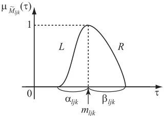
j is the Gaussian random variable with fuzzy mean value Mljk which is represented by an L-R fuzzy number characterized by the membership function
if
if ,
ljk
ljk
ljk ljk
M
ljk
ljk ljk
m
L m
m
R m
(3)
where the shape functions L and R arenonincreasing con-tinuous functions from 0,
to
0,1 , ljk is themean value, and ljk
m
and ljk are positive numbers
which represent left and right spreads. Figure 1 illus- trates an example of the membership function
ljk
M
.
Let Γ be a collection of all possible Gaussian random variables N s
,2
where s
,
and 2
0,
. Then, Cljk is expressed as a random fuzzy vari- able with the membership function
~
, 2
, Γ.ljk
ljk ljk M ljk ljk ljk ljk ljk
C s N s
(4) Through the Zadeh’s extension principle, in view of (4), the membership function of a random fuzzy variable cor- responding to each of objective functions zl
x x1, 2
,1, 2
l is given as
0 1
L R
μ Mljk (~ τ)
αljk βljk
mljk
[image:3.595.348.531.310.378.2]τ
Figure 1. An example of the membership function
ljk
[image:3.595.343.503.597.710.2]
2
1 , 1,2 1 1
2
1 , 1,2 1 1
sup min
sup min ~ ,
j l l j ljk
j ljk
j l
n
l k n j C ljk l ljk jk
j k n
ljk l ljk jk l M
k n j
s j k
u u
s u N s x V
C x
x
x
(5) where l
l11, ,l n11,l21,,l n22
,
11, , 11, 21, , 22
l l l n l l n
s s s s s
2 nj
, and
2 21 1
.
l ljk jk j k
V x
x
4. Fractile Criteria with Possibility
Incorporating Fuzzy Goals
Assuming that the decision makers (DMs) concerns about the probabilities that their own objective function values
l
C x are smaller than or equal to certain target values , we introduce the probabilities
, 1, 2
l f l
lP C x fl
which are expressed as fuzzy setsl
P with the membership functions
sup
,l
l l u l l l l l
P p u p P u f
C x
(6)
where are the initial target values specified by the DMs as constants. f ll, 1, 2
Considering the imprecise nature of the DMs’ judg-ments for the probabilities l with respect to the ran-dom fuzzy objective values
P
, 1, 2
l l
C x
, 2
, we introduce the fuzzy goals G ll such as “ l should be
greater than or equal to a certain value.’’ Such fuzzy goals can be quantified by eliciting corre-sponding membership functions
, 1
P
, 1, 2
l
G l
0
0 1
1
0 if
if , 1, 2.
1 if
l
l
l l l
G
l
p p
p g p p p p l
p p
l
(7)
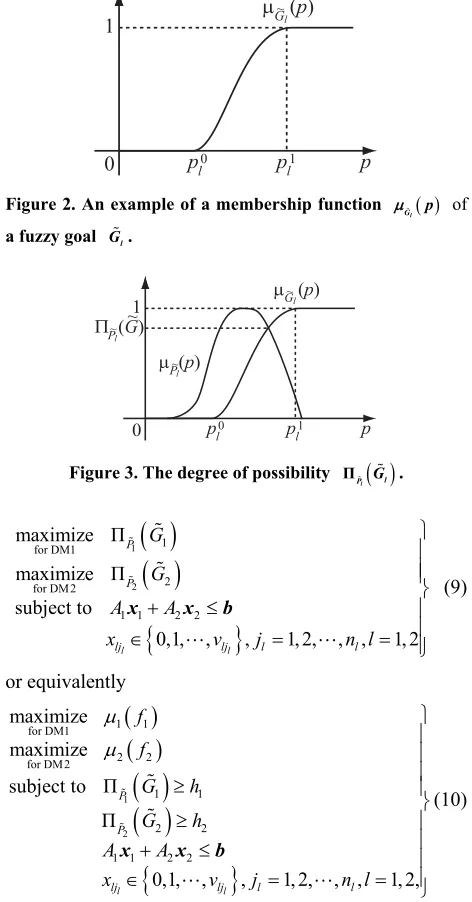
where are nondecreasing functions. Fig-ure 2 illustrates a possible shape of the membership func- tion for the fuzzy goal .
, 1, 2l
g p l
l
Recalling that the membership function is regarded as a possibility distribution, the degree of possibility that the probability attains the fuzzy goal is expressed as
G
l
P Gl
Π sup min , , 1, 2.
l
l l p l l l l
[image:4.595.337.491.83.179.2] [image:4.595.57.290.86.238.2]P G P p G p (8)
Figure 3 illustrates the degree of possibility Π
Gl l
P Now, assuming that the DMs are willing to maximize the degrees of possibility with respect to the attained prob- ability, we consider the possibility-based probability model for random fuzzy two-level programming problems for- mulated as
.
0 1
pl1
pl0 p
μ (Gl~ p)
Figure 2. An example of a membership function
l
G p
of
a fuzzy goal Gl.
0 1
pl1
pl0 p
μ (G~l p)
[image:4.595.305.541.90.541.2]μ (P~lp) ΠP (~l G~)
Figure 3. The degree of possibility ΠPl
Gl .
1
2
1 for DM1
2 for DM2
1 1 2 2
maximize Π maximize Π subject to
0,1, , , 1, 2, , , 1, 2
l l
P P
lj lj l l
G
G
A A
x v j n l
x x b
(9)
or equivalently
1
2 1 1 for DM1
2 2 for DM2
1 1
2 2
1 1 2 2
maximize maximize
subject to Π
Π
0,1, , , 1, 2, , , 1, 2,
l l
P P
lj lj l l
f f
G h
G h
A A
x v j n l
x x b
(10)
where 1 and 2 are permissible possibility levels
specified by the DMs, and 1
h h
and 2 are the mem-
bership functions of the fuzzy goals for the target vari- ables f1 and f2, respectively.
It should be noted here that the bilevel programming problem (10) involves the possibility constraints
ΠPl Gl h ll, 1, 2. Fortunately, however, the
follow-ing theorem holds for the constraints
in (10).
Π , 1, 2
l l l
P G h l
Theorem 1. Let denoteaprobabilitydistribution
functionofthestandard GaussianrandomvariableN(0,
1). Then,
Φ
ΠPl ,l1, 2 in (10) is equivalently
transformedinto l l
G h
2
1
1 1
Φ ,
j
l
n
ljk l ljk jk G l l l j k
m L h x h V x f
where L h
l isa pseudoinverse functionsdefined as
sup
Φ1Φ
2 1 1 ~ , j nl ljk l ljk jk l
j k
u N m L h x V
x , (13)
, 0
L h t L t h r
l l and is the inverse
functionof .
Since P
ul
f
Proof
l is transformed into
From (8), the constraints
l l l
P in (10)
is equivalently replaced by the condition that there exists a p such that
Π G h l, 1, 2
l l
P p hl
and Gl
pl hl, namely,
2 1 1 2 1 1 j j nl j k ljk l ljk jk l
n
l j k ljk l ljk jk l
u m L h
P
V
f m L h x
V x
x x
1 , 1,2
2
1 1
sup min ,
~ , 1 ljk j l j
ljk l l l M
k n j n
l ljk jk l l j k
s p P u f
u N s x V h
s x (11)in consideration of and
l
l G l , where are pseudo inverse functions defined as
, 1, 2
p h l
l l G h
2 1 1 ~ 0,1 j nl j k ljk l ljk jk l
u m L h x
N V
x ,
inf
, 1, 2l l l l l l
G h p G p h l
. This implies that
(13) isequivalently transformed as there exists a vector
p s ul, ,l l
,l1, 2 such that
2
1 min, 1,2 , ~ 1 1 , ,
j ljk
j
n
ljk l l ljk jk l M
k n j s h u N j k s x V
x
2 1 1 Φ , j l nl j k ljk l ljk jk G l
f m L h x
V
x (14)
,l
l l l l G
p P u f p , where is a probability distribution function of the standard Gaussian randomvariable .
Φ
0,1N Φ whichcan be equivalently transformed into the condition
that there exists a vector
s ul, l
such that written as From the monotone increasingnessof , (14) isre-
2
1 1
, ~ , ,
j ljk
n
ljk l l ljk jk l M
j k
s h u N s x V
x
2 1 1 1 Φ j l nljk l ljk jk G l l l j k
m L h x h V f
x(15)
, 1, 2, 1, 2, 1, ,l
l l G j
P u f l j k n . (12)
where Φ1 is the inverse function of Φ.
From (11)-(15), it holds that In view of (3), it follows that
ljk ljk l
M s h
,
ljk ljk l ljk ljk l ljk
s m L h m R h
,
2 1 1 1 Π Φ . l j l l l P nljk l ljk jk G l l l j k
G h
m L h x h V f
x
(16) where L h
l and R h
l
are pseudo inverse func- tions defined asL hl sup
t L t
hl
and
This completes the proof of the theorem.
l
l
R h sup t L t h . Hence, (12) is rewritten as
Due to Theorem 1, the two-level integer programming problem with the possibility constraints (9) is equiva- lently transformed into (17)
theequivalent condition that there exists a ul such that
,l
l l l G
P u f p , or equivalently (18)
1 2 1 1 for DM1 2 2 for DM2 2 11 1 1 1 1 1 1
1 1
2
1
2 2 2 2 2 2
1 1
1 1 2 2
maximize maximize
subject to Φ
Φ
0,1, , , 1, 2, , , 1, 2,
j j
l l
n
jk jk jk G
j k n
jk jk jk G
j k
lj lj l l
f f
m L h x h V f
m L h x h V f
A A
x v j n l
x xx x b
Π,1 1 1 2
for DM1
Π,
2 2 1 2
for DM2
1 1 2 2
maximize ,
maximize ,
subject to
0,1, , , 1, 2, , , 1, 2,
l l
F F
lj lj l l
Z Z
A A
x v j n l
x x x x
x x b
(18) where
2 Π, 1 2 1 1 1 ,Φ , 1, 2
j
l
n F
l ljk l ljk jk
j k
l l
G
Z m L h
h V l
x x x . x (19)It should be emphasized here that (18) is a determinis-tic two-level nonlinear integer programming problem.
5. Interactive Fuzzy Programming
In order to obtain an initial candidate for an overall sat-isfactory solution to (9) or (17), it would be useful for DM1 to find a solution which maximize the smallerde-gree of satisfaction between the two DMs by solving the maximin problem
Π, Π,
1 1 1 2 2 2 1 2
1 1 2 2
maximize min , , ,
subject to
0,1, , , 1, 2, , , 1, 2,
l l
F F
lj lj l l
Z Z
A A
x v j n l
x x x x
x x b
(20) By introducing an auxiliary variable , this problem is written as
Π,1 1 1 2
Π,
2 2 1 2
1 1 2 2
maximize
subject to ,
,
0,1, , , 1, 2, , , 1, 2,
l l
F F
lj lj l l
v
Z v
Z v
A A
x v j n l
Although the membership function does not always need to be linear, for the sake of simplicity, we adopt a linear membership function which characterizes the fuzzy goal of each decision maker. The linear membership func-tions l,l1, 2 are defined as
Π, 1 2Π, 1
1 2
Π, 0
1 2 1 Π, 0
1 2
1 0
Π, 0
1 2
,
1 if ,
,
if ,
0 if ,
F l l
F
l l
F
l l F
l l l
l l F l l Z Z z Z z
z Z z
z z Z z . x x x x x x x x x x (22)
Then, (21) is equivalently transformed as (23)
If DM1 is satisfied with the membership function val- ues
Π,
1, 2 , 1,
F
l Zl l
x x 2, the corresponding opti
mal solution x to (21) is regarded as the
satisfactory-solution. Otherwise, by introducing the constraint that
Π,
1 Z1 F
x is larger than or equal to the minimal sat-isfactory level
0,1 specified by DM1, we con-sider the problem of maximizing the membership func-tion
Π,
2
2 Z2 F
x x1, formulated as
2 2 1 2
Π,
1 1 1 2
1 1 2 2
maximize ,
subject to ,
0,1, , , 1, 2, , , 1, 2,
l l
F
lj lj l l
Z Z
A A
x v j n l
Π,F
x x x x
x x b
(24)
x x x x
x x b
(21)
or equivalently (25)
In general, when the objective functions of DM1 and DM2 conflict with eachother, it should be noted here that the larger the minimal satisfactory level δ for 1 is
spe-cified by DM1, the smaller the satisfactory degree for
2
becomes, whichmay lead to the improper satisfac-
1 2 21 1 0
1 1 1 1 1 1 1 1
1 1
2
1 1
2 2 2 2 2 2 2
1 1
1 1 2 2
maximize
subject to Φ
Φ
0,1, , , 1, 2, , , 1, 2,
j j
l l
n
jk jk jk G
j k n
jk jk jk G
j k
lj lj l l
v
m L h x h V z z v z
m L h x h V z z v z
A A
x v j n l
x xx x b
0 0 0 2
(23)
2 1 2 12 2 2 2 2
1 1 2
1 1
1 1 1 1 1 1 1
1 1
1 1 2 2
maximize Φ
subject to Φ
0,1, , , 1, 2, , , 1, 2,
j j
l l
n
jk jk jk G j k
n
jk jk jk G j k
lj lj l l
m L h x h V
m L h x h V z z z
A A
x v j n l
x xx x b
0 0
1
tory balance between DM1 and DM2 due to the large difference between the membership function values of both DMs.
In order to derive the satisfactory solution which has well-balanced membership function values between both DMs, by introducing the ratio Δ expressed as
Π,
2 2 1 2
Π,
1 1 1 2
,
Δ ,
, F F
Z Z
x x
x x (26) the lower bound min and the upper bound of max of
, specified by DM1, are introduced to determine whe- ther or not the ratio Δ is appropriate. To be more explicit, if it holds that
Δ Δ
Δ
min max
Δ Δ ,Δ ,
then DM1 regards the corresponding solution as a pref- erable candidate for the satisfactory solution with well- balanced membership function values.
Now we summarize a procedure of interactive fuzzy programming through fractile criteria with possibility in order to derive a satisfactory solution.
Interactive Fuzzy Programming through Fractile Criteria with Possibility
Step 0: Ask DMs to specify the initial target values , and determine the membership functions , 1, 2
l
f l
, 1,
l
G l 2
.
Step 1: Ask DM1 to specify the permissible possibil-ity levels h ll, 1, 2.
Step 2: Ask DMs to determine the membership func- tions l,l 1, 2.
Step 3: For the current , solve the maxmin problems (20).
, 1, l
h l 2
Step 4: DM1 is supplied with the current values of the membership functions 1 and 2 for the optimal so-
lution obtained in step 3. If DM1 is satisfied with the current membership function values, then stop. If DM1 is not satisfied and prefers to update , ask DM1 to update l, and return to step 3. Otherwise, ask DM1 to specify the minimal satisfactory level
, 1, l
h l 2
h
for
Π, 1 Z1 F x
and the permissible range
Δmin,Δmax
of the ratio Δ.
Step 5: For the current minimal satisfactory level δ, solve the membership function maximization problem (25).
Step 6: DM1 is supplied with the current values of the membership function 1, 2 and the ratio Δ. If
min max
Δ Δ ,Δ and DM1 is satisfied with the current membership function values, then stop. Otherwise, ask DM1 to update the minimal satisfactory level δ, and re- turn to step 5.
In the proposed interactive fuzzy programming method, it is required to solve the nonlinear integer programming
problems (20) and (25), which is apparently difficult to solve compared to linear integer programming problems and 0-1nonlinear programming problems. In order to solve such difficult problems, in the following section, we introduce genetic algorithms designed for nonlinear integer programming problems.
6. Genetic Algorithms for Nonlinear Integer
Programming
For solving linear integer programming problems on the framework of geneticalgorithms, Sakawa proposed GADSLPRRSU [29]. GADSLPRRSU is an abbreviation for genetic algorithms with double strings based on linear programming relaxation and reference solution updating. This method includes three key ideas: double strings (DS), linear programming relaxation (LPR), and reference so-lution updating (RSU). Unfortunately, however, due to nonlinearity, we cannot directly apply GADSLPRRSU for solving (20) and (25). However, we can introduce the revised GADSLPRRSU where GENOCOPIII [30,31] is employed for solving a nonlinear continuous relaxation problem.
As an efficient approximate solution method, the re- vised GADSLPRRSU are designed for nonlinear integer programming problems formulated as:
minimize
subject to 0, 1, 2, , 0,1, , , 1, 2, , i
j j
f
g i m
x v j n
x x
(27)
where is an dimensional integer decision vari-able column vector. Furthermore,
x n
f and
, 1, 2,i ,
g i m may be nonlinear.
Quite similar to genetic algorithms with double (GADS) [29], an individual is represented by a double string shown in Figure 4. In Figure 4, for a certain j s j,
1, 2,,n
represents an index of decision variable xs j in the solution space, while does the inte- ger value among , 1, s j
y j 2, , n
0,1, , vj
of the s j
th decisionvariable xs j .
Now we can summarize the computational procedures of the revised GADSLPRRSU as follows.
Computational Procedures of the Revised GADSLPRRSU
Step 0: Determine values of the parameters used in the genetic algorithm. Set the generation counter at 0. t
Step 1: Generate the initial population consisting of
s(1) s(2) ··· s(n)
ys(1) ys(2) ··· ys(n)
N individuals based on the information of the optimal
solution to the continuous relaxation problem.
Step 2: Decode each individual in the current popula- tion and calculate its fitness based on the corresponding solution.
Step 3: If the termination condition is fulfilled, stop. Otherwise, let t: t 1.
Step 4: Apply reproduction operator using elitist ex- pected value selection after linear scaling.
Step 5: Apply crossover operator, called PMX (Par- tially Matched Crossover) for double string.
Step 6: Apply mutation based on the information of a solution to the continuous relaxation problem.
Step 7: Apply inversion operator, return to Step 2. Further details of GADSLPRRSU and the revised GADSLPRRSU can be found in [17,29,32].
7. Numerical Example
To demonstrate the feasibility and efficiency of the pro- posed method, consider the following two-level integer programming problem involving random fuzzy variable coefficients:
2
1 1 2 11 1 12 2
for DM1
2 1 2 21 1 22 2
for DM2
11 1 12 2 1
21 1 22 2 2
31 1 32 2 3
41 1 42 2 4
51 1 52 2 5
2
minimize ,
minimize ,
subject to
0,1, ,30 , 1, 2,3, 1, 2. lj
z
z
a a b
a a b
a a b
a a b
a a b
x j l
x x C x C x
x x C x C x
x x
x x
x x
x x
x x
[image:8.595.349.494.307.369.2](28)
Table 1 shows values of coefficients of constraints and and Table 2 shows , 1, 2,3, 4,5
i
[image:8.595.65.287.361.497.2]a i b ii, 1, 2,3, 4,5
Table 1. Values of coefficients in constraints.
al11 al12 al13 al21 al22 al23 b
a1 15.00 20.00 20.00 0.00 0.00 0.00 1400
a2 0.00 0.00 0.00 2.50 9.00 4.00 430
a3 5.00 2.00 1.00 5.00 5.00 8.00 400
a4 3.00 8.00 4.00 7.00 8.00 8.00 600
a5 3.50 4.00 4.00 5.50 4.00 1.00 300
Table 2. Values of mljk, αljk and σljk. 2
11
l
c cl12 cl13 cl21 cl22 cl23
m1jk 7.00 4.00 5.00 3.00 5.00 3.00
m2jk 4.00 3.00 4.00 2.00 4.00 3.00
a1jk 0.70 0.50 0.80 0.40 0.70 0.60
a2jk 0.90 0.80 0.70 0.40 0.60 0.50
2 1jk
1.40 1.00 1.10 1.20 1.10 0.90
2 2jk
values of parameters of random fuzzy variables ljk, ljk
m
and , where train-
gular fuzzy numbers are assumed for
2, 1, 2, 1, 2, 1, 2, ,6
ljk l j k
ljk
M
.
Through the use of this numerical example, it is now appropriate to illustrate the proposed interactive fuzzy programming.
For illustrative purposes, assume that DMs specify the initial target values as f1 120.00 and f290.00
and determine the membership functions (7) for the prob- abilities and as linear ones by assessing
, , , and
1 P
50 2
P
0.
0 1 0.
p 0
2 40
p 1
1 0.85
p 1
2 p 0.80
1 2
0.5 0.4
, .
0.35 0.4
p p
g p g p
Also assume that DM1 specify the permissible possi- bility levels as h10.7 and 2 . Furthermore,
assume that the fuzzy goals for the target variables 1
0.7
h
f
and f2 are determined by the linear membership functions
1
0
1 0
1 0
0
1 if
if
0 if .
l l l l
l l l l l
l l
l l
f f
f f
f f f f
f f
f f
where the parameter values characterizing the linear membership functions are determined as ,
, , and .
1
1 131.65
f
16.95
0.7
h
0
1 69.26
f 1
2 93.91
f 0
2 f
For the permissible possibility levels of 1 and
2 0.7
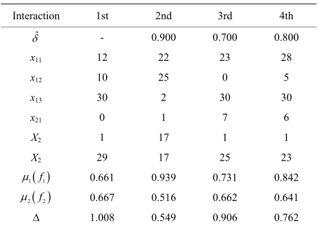
h , the corresponding maximin problem (20) is solved through the revised GADSLPRRSU, and the ob- tained result is shown at the column labeled “1st”in Ta-ble 3. DM1 is not satisfied with this solution, but he does not desire to update ,h ll 1, 2. Thus, DM1 determines the minimal satisfactory level ˆ 0.90 to improve
1 f1
at the expense of 2
f2 Δ. Furthermore, DM1 specifies the upper bound max and the lower
bound
0.90
min 0.60
Δ for the ratio of membership func-tions Δ2
f2 1
f1 .Table 3. Interaction process.
Interaction 1st 2nd 3rd 4th
ˆ
- 0.900 0.700 0.800
x11 12 22 23 28
x12 10 25 0 5
x13 30 2 30 30
x21 0 1 7 6
X2 1 17 1 1
X2 29 17 25 23
1 f1
0.661 0.939 0.731 0.842
2 f2
0.667 0.516 0.662 0.641
Δ 1.008 0.549 0.906 0.762
[image:8.595.307.540.568.734.2]For the updated value of ˆ , the corresponding prob- lem (25) is solved by the revised GADSLPRRSU. The obtained result is shown at the column labeled “2nd”in
Table 3. Since the ratio of satisfactory degrees Δ is less than min , the second condition of termination of
the interactive process is not fulfilled. Hence, DM1 up- dates the minimal satisfactory level
Δ 0.60
ˆ
from 0.90 to 0.70 for improving 2
f2 at the sacrifice of 1
f1 . For the updated value of ˆ , the corresponding (25) is solved, and the obtained result is shown at the column labeled “3rd” in Table 3. DM1 considers that 1
f1 is improved but is greater than max. Hence, DM1 isnot satisfied with this solution and updates the minimal satisfactory level
Δ Δ
ˆ
from 0.70 to 0.80. For the updated value of ˆ , the corresponding (25) is solved, and the obtained result is shown at the column labeled “4th” in
Table 3. Since Δ exists in the interval
min
andDM1 satisfied with the balance between max
Δ ,Δ
1 f1
and
22 f
, the interactive algorithm is terminated.
In the proposed interactive fuzzy nonlinear program- ming, through a series of update procedures of the mini- mal satisfactory level ˆ , it can be possible to obtain a satisfactory solution where the satisfactory degree of DM1 is guaranteed to be greater than or equal to the minimal satisfactory level ˆ and is well balanced with that of DM2.
8. Conclusion
In this paper, for tackling cooperative decision making problems in hierarchical organizations under random fuzzy environments, we introduced fuzzy two-level inte- ger programming problems involving random fuzzy vari- ables. Considering the probabilities that the decision mak- ers’ objective function values are smaller than or equal to target variables, fuzzy goals of the decision makers for the probabilities were introduced. Through the use of fractile criteria in stochastic programming, the original random fuzzy two-level programming problems were reduced to deterministic ones. In order to obtain a satis- factory solution for the decision maker at the upper level in consideration of the cooperative relation between deci- sion makers, interactive fuzzy programming for random fuzzy two-level integer programming problems was pro- posed. It was shown that all of the problems to be solved in the proposed interactive fuzzy programming can be solved through genetic algorithms for nonlinear integer programming, called the revised GADSLPRRSU. An il- lustrative numerical example demonstrated the feasibility and efficiency of the proposed method. Extensions to other stochastic programming models will be considered elsewhere. Also extensions to noncooperative environments will be required in the near future.
REFERENCES
[1] K. Shimizu, Y. Ishizuka and J. F. Bard, “Nondifferenti- able and Two-Level Mathematical Programming,” Klu- wer Academic Publishers, Boston, 1997.
doi:10.1007/978-1-4615-6305-1
[2] M. Sakawa and I. Nishizaki, “Cooperative and Noncoop- erative Multi-Level Programming,” Springer, New York, 2009.
[3] W. F. Bialas and M. H. Karwan, “Two-Level Linear Pro- gramming,” ManagementScience, Vol. 30, No. 8, 1984, pp. 1004-1020. doi:10.1287/mnsc.30.8.1004
[4] I. Nishizaki and M. Sakawa, “Computational Methods through Genetic Algorithms for Obtaining Stackelberg Solutions to Two-Level Mixed Zero-One Programming Problems,” Cybernetics and Systems: An International
Journal, Vol. 31, No. 2, 2000, pp. 203-221.
doi:10.1080/019697200124892
[5] M. Simaan and J. B. Cruz Jr., “On the Stackelberg Strat- egy in Nonzero-Sum Games,” Journal of Optimization
TheoryandApplications, Vol. 11, No. 5, 1973, pp. 533-
555. doi:10.1007/BF00935665
[6] Y. J. Lai, “Hierarchical Optimization: A Satisfactory So- lution,” FuzzySetsandSystems, Vol. 77, No. 3, 1996, pp. 321-325. doi:10.1016/0165-0114(95)00086-0
[7] H. S. Shih, Y. J. Lai and E. S. Lee, “Fuzzy Approach for Multi-Level Programming Problems,” Computers and
OperationsResearch, Vol. 23, No. 1, 1996, pp. 73-91.
doi:10.1016/0305-0548(95)00007-9
[8] M. Sakawa, I. Nishizaki and Y. Uemura, “Interactive Fuzzy Programming for Multi-Level Linear Programming Pro- blems,” Computers & Mathematics with Applications, Vol. 36, No. 2, 1998, pp. 71-86.
doi:10.1016/S0898-1221(98)00118-7
[9] M. Sakawa, I. Nishizaki and Y. Uemura, “Interactive Fuzzy Programming for Multi-Level Linear Fractional Pro- gramming Problems with Fuzzy Parameters,” FuzzySets
andSystems, Vol. 109, No. 1, 2000, pp. 3-19.
doi:10.1016/S0165-0114(98)00130-4
[10] M. Sakawa, I. Nishizaki and Y. Uemura, “Interactive Fuzzy Programming for Two-Level Linear and Linear Fractional Production and Assignment Problems: A Case Study,” Eu-
ropeanJournalofOperationalResearch, Vol. 135, No. 1,
2001, pp. 142-157. doi:10.1016/S0377-2217(00)00309-X [11] M. Sakawa and I. Nishizaki, “Interactive Fuzzy Program-
ming for Decentralized Two-Level Linear Programming Problems,” FuzzySetsandSystems, Vol. 125, No. 3, 2002, pp. 301-315. doi:10.1016/S0165-0114(01)00042-2 [12] M. Sakawa, I. Nishizaki and Y. Uemura, “A Decentral-
ized Two-Level Transportation Problem in a Housing Ma- terial Manufacturer: Interactive Fuzzy Programming Ap-proach,” EuropeanJournalofOperationsResearch, Vol. 141, No. 1, 2002, pp. 167-185.
doi:10.1016/S0377-2217(01)00273-9
[13] M. Sakawa, I. Nishizaki and Y. Uemura, “Interactive Fuzzy Programming for Two-Level Linear Fractional Program- ming Problems with Fuzzy Parameters,” Fuzzy Setsand
Systems, Vol. 115, No. 1, 2000, pp. 93-103.
[14] M. Sakawa and I. Nishizaki, “Interactive Fuzzy Program- ming for Two-Level Nonconvex Programming Problems with Fuzzy Parameters through Genetic Algorithms,” Fuzzy
SetsandSystems, Vol. 127, No. 2, 2002, pp. 185-197.
doi:10.1016/S0165-0114(01)00134-8
[15] M. Sakawa and H. Katagiri, “Interactive Fuzzy Program- ming Based on Fractile Criterion Optimization Model for Two-Level Stochastic Linear Programming Problems,”
CyberneticsandSystems, Vol. 41, No. 7, 2010, pp. 508-
521. doi:10.1080/01969722.2010.511547
[16] M. Sakawa and K. Kato, “Interactive Fuzzy Programming for Stochastic Two-Level Linear Programming Problems through Probability Maximization,” InterimReport, IR- 09-013, International Institute for Applied Systems Ana- lysis (IIASA), 2009.
[17] M. Sakawa, H. Katagiri and T. Matsui, “Interactive Fuzzy Stochastic Two-Level Integer Programming through Frac- tile Criterion Optimization,” Operational Research: An
InternationalJournal, Vol. 12, No. 2, 2012, pp. 209-227.
doi:10.1016/S0377-2217(01)00273-9
[18] M. Sakawa, H. Katagiri and T. Matsui, “Interactive Fuzzy Random Two-Level Linear Programming through Frac- tile Criterion Optimization,” MathematicalandComputer
Modelling, Vol. 54, No. 11-12, 2011, pp. 3153-3163.
doi:10.1016/j.mcm.2011.08.006
[19] M. Sakawa, I. Nishizaki and H. Katagiri, “Fuzzy Stochas- tic Multiobjective Programming,” Springer, New York, 2011. doi:10.1007/978-1-4419-8402-9
[20] H. Kwakernaak, “Fuzzy Random Variables. I. Definitions and Theorems,” Information Sciences, Vol. 15, No. 1, 1978, pp. 1-29. doi:10.1016/0020-0255(78)90019-1 [21] M. L. Puri and D. A. Ralescu, “Fuzzy Random Variables,”
JournalofMathematicalAnalysisandApplications, Vol.
114, No. 2, 1986, pp. 409-422. doi:10.1016/0022-247X(86)90093-4
[22] G.-Y. Wang and Z. Qiao, “Linear Programming with Fuzzy Random Variable Coefficients,” Fuzzy Sets and Systems, Vol. 57, No. 3, 1993, pp. 295-311.
doi:10.1016/0165-0114(93)90025-D
[23] M. Sakawa and I. Nishizaki, “Interactive Fuzzy Program- ming for Multi-Level Programming Problems: A Re-
view,” International Journal of Multicriteria Decision
Making, Vol. 2, No. 3, 2012, pp. 241-266.
doi:10.1504/IJMCDM.2012.047846
[24] B. Liu, “Random Fuzzy Dependent-Chance Programming and Its Hybrid Intelligent Algorithm,” Information Sci-
ences, Vol. 141, No. 3-4, 2002, pp. 259-271.
doi:10.1016/S0020-0255(02)00176-7
[25] M. Sakawa and T. Matsui, “Interactive Fuzzy Program- ming for Random Fuzzy Two-Level Programming Prob- lems through Possibility-Based Fractile Model,” Expert
SystemswithApplications, Vol. 39, No. 16, 2012, pp. 12599-
12604. doi:10.1016/j.eswa.2012.05.024
[26] A. M. Geoffrion, “Stochastic Programming with Aspira- tion or Fractile Criteria,” Management Science, Vol. 13, No. 9, 1967, pp. 672-679. doi:10.1287/mnsc.13.9.672 [27] M. A. Gil, M. Lopez-Diaz and D. A. Ralescu, “Overview
on the Development of Fuzzy Random Variables,” Fuzzy
SetsandSystems, Vol. 157, No. 19, 2006, pp. 2546-2557.
doi:10.1016/j.fss.2006.05.002
[28] S. Nahmias, “Fuzzy Variables,” FuzzySetsandSystems, Vol. 1, No. 2, 1978, pp. 97-110.
doi:10.1016/0165-0114(78)90011-8
[29] M. Sakawa, “Genetic Algorithms and Fuzzy Multiobjec- tive Optimization,” Kluwer Academic Publishers, Boston, 2001.
[30] S. Koziel and Z. Michalewicz, “Evolutionary Algorithms, Homomorphous Mapping, and Constrained Parameter Op- timization,” Evolutionary Computation, Vol. 7, No. 1, 1999, pp. 19-44. doi:10.1162/evco.1999.7.1.19
[31] Z. Michalewicz and G. Nazhiyath, “GenocopIII: A Co- Evolutionary Algorithm for Numerical Optimization Pro- blems with Nonlinear Constraints,” Proceedings of the
Second IEEE International Conference onEvolutionary
Computation,Perth, 29 November-1 December 1995, pp.
647-651.
[32] M. Sakawa, K. Kato, M. A. K. Azad and R. Watanabe, “A Genetic Algorithm with Double String for Nonlinear Integer Programming Problems,” Proceedings of 2005
IEEEInternationalConferenceonSystems, ManandCy-