Texture Feature Extraction for Identification of
Medicinal Plants and Comparison of Different
Classifiers
C. H. Arun
Department of Computer Science NMC College
Marthandam, India
W. R. Sam Emmanuel
Department of Computer ScienceNMC College Marthandam, India
D. Christopher Durairaj
Department of Computer ScienceVHNSN College Virudhunagar, India
ABSTRACT
This paper presents an automated system for recognizing the medicinal plant leaves that are taken from the suburbs of the western ghats region. The dataset comprises of 250 different leaf images, of five species. Texture analyses of the leaf images have been done in this work using the feature computation. The features include grey textures, grey tone spatial dependency matrices(GTSDM) and Local Binary Pattern(LBP) operators. For each leaf image, a feature vector is generated from the statistical values. 70% of the images in the dataset are the training dataset and the rest are included in the test set. Six different classifiers are used to classify the plant leaves based on feature values. When features are combined without any preprocessing, it yielded a classification performance of 94.7%.
General Terms:
image processing, pattern recognition
Keywords:
image classification, texture features, plant identification
1. INTRODUCTION
Herbal medicines are gaining popularity worldwide as they are safe to human health and affordable. World Health Organization estimates that 80% of people in Asia and Africa rely on herbal medicines for some aspects of their primary health care [1]. There are diverse medicinal plant varieties in lush forests of southern india which are used as medicines to a number of sicknesses like common cold, allergies etc. Precise identification of the respective plant leaf is vital in treating the patients. The present work explores the use of texture features to identify the appropriate medicinal leaves automatically.
Textures are a pattern of non-uniform spatial distribution of differing image intensities [11], which focus mainly on the individual pixels that make up an image. Texture is defined by quantifying the spatial relationship between materials in an image. Texture analyses is done by using various approaches like statistical, fractal, and structural. Statistical type includes techniques like grey-level histogram, grey-level co-occurence matrix [20], local binary pattern operator, auto-correlation features and power spectrum.
Grey texture features or the first order statistical features are used in image classification [15]. Haralick et al [14], described texture features based on grey-level co-occurence
matrix(GLCM) and are used in various applications including Land cover classification [22]. Ojala et al [19] used texture feature based on local binary pattern(LBP).
Textures are useful in identifying plant leaves without the need for an expert. [26][21][12]. Plant leaves are recognized based on the features of leaf images[7]. Classification of leaf epidermis microphotographs is done using texture features [23]. Basavaraj et al [3], Sandeep et al [24] identified medicinal plant leaves using textures.
Classification approaches like Stochastic Gradient Descent(SGD) [25][18] , kNearest Neighbour(kNN) [4][2], Support Vector Machines(SVM) [10], Decision Trees(DT) [5], Extra Trees(ET) [13], Random Forests(RF)[8][6] can be used as Image classifiers.
The objective of the present work is to compute texture features based on grey-level, the Grey Tone Spatial Dependency Matrix(GTSDM) and the Local Binary Pattern(LBP) operators and to obtain the best combination of these, for automatically identifying the right medicinal plant.
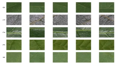
Five medicinal plant leaves are considered and few of their medicinal uses are given below. A sample of the medicinal plant leaf dataset from different plant leaves are given in Fig. 1.
(0) Desmodium gyrans - Antidote for snake poison, effective for heart diseases, rhematic complaints, Diabetes and skin ailments.
(1) Butea monosperma - promotes diuresis and anthelmintic, treats leucorrhea and diabetes.
(2) Malpighia glabra - help lower blood sugar, increases collagen and elastin production, treats diarrhea, dysentery, and liver problems.
(3) Helicteres isora- help treat intestinal complaints, colic pains and flatulence.
(4) Gymnema sylvestre - suppresses the sensation of sweet, anti-diabetic.
Fig. 1. Leaf images of Desmodium gyrans (row 0), Butea monosperma (row 1), Malpighia glabra (row 2), Helicteres isora
(row 3)and Gymnema sylvestre (row 4)
2. METHODOLOGY 2.1 Texture Features
The different Texture features namely, Grey-level, GTSDM based second-order and LBP features are briefly presented in this section.
2.1.1 Grey Textures. One of the simplest texture descriptors is first-order statistical central moments which are also referred as Gray level features. They include mean, variance, skewness and standard deviation. First order features do not take relative layout between gray values into account.
Thexibe a random variable which denotes the gray levels in an image and L be the number of distinct gray levels, thenP(xi)is defined as the probability of occurence of pixels with intensity xias in Eqn.(1).
P(xi) =
k
N (1)
wherekis the number of pixels with grey levelxiand N is the total number of pixels in the region.
Mean(µ0), the first of the grey-level feature, which averages the gray levels of the image is defined as in Eqn.(2).
µ0 = L−1
X
i=0
xiP(xi) (2)
Variance(µ2) is referred as the second moment which is a measure of gray-level contrast that are used to describe the descriptors of relative smoothness. Variance is defined as in Eqn.(3). Variance values tend to be larger for images with values.
µ2 = L−1
X
i=0
(xi−µ0)P(xi) (3)
The third moment is a measure of skewness(µ3) of the histogram as in Eqn.(4). The third moment will be of use only when the variations between measurements are too large.
µ3 = L−1
X
i=0
(xi−µ0)2P(xi) (4)
Standard Deviation(σ) can also be used as a measure of texture and is defined as in Eqn.(5).
σ= v u u t 1 L
L−1
X
i=0
(P(xi)−µ0)2 (5)
00 450 900
[image:2.595.77.272.107.222.2]1350
Fig. 2. Theθorientations for feature computation
2.1.2 GTSDM Based Textures. Grey Tone Spatial Dependency Matrix(GTSDM) features are second-order features and are usually more sensitive and intuitive than first-order measures. GTSDM texture features are based on the GTSD matrix. The texture is related with the statistical distribution of gray tones. The GTSDM is a tabulation of probability of grey levels i occuring in an image at a distancedin angle θfrom grey level jat points from p1(x1, y1) to p2(x2, y2). These probabilities create the co-occurence matrix as of Eqn.(6).
G=P(i,j|d, θ) (6)
The distance and the angle are obtained as given in Eqn. (7) and Eqn. (8) and the different directions of adjacency for calculation the texture feature is given in Fig. 2
d(p1,p2) =
q
(x2−x1) 2
+ (y2−y1) 2
(7)
θ(p1,p2) =tan−1
(y2 −y1)
(x2 −x1)
(8)
By computing the frequency of one grey tone to the neighbourhood of others, a k x k matrix is formed. The frequencies of the reference and neighbour grey-tones constituting a pair in the colour image is computed. The (i,j)th element of GTSDM matrix G is computed by finding the frequency of the neighbour grey-tonej occuring near the reference grey-toneiwithin the colour image. In order to make the generated matrix independent of the direction, the matrix G is transposed (G0) to make it symmetrical(S), which is defined in Eqn.(9).
S =G+G0 (9)
The Symmetrical GTSDM is then normalised by dividing each element by the sum of all the elements as in Eqn.10 to formSθ, whereθis the angle which varies as 0, 45, 90 and 135 as shown in Fig. 2. This represents the directions along horizontal(θ= 0◦
), right diagonal (θ= 45◦), vertical (θ= 90◦
) and the left-diagonal (θ= 135◦
).
Sθ=
S X
i
X
j
Sij
(10)
Feature Extraction
Training Set Data Set
Testing Set
Classifiers
SGD KNN SVM DT ET RF
[image:3.595.94.245.91.243.2]Classified Image
Fig. 3. Block diagram for Classification
entropy. Entropy is defined as in Eqn.(11). The termSijin the equation represent the element(i,j)of a normalised symmetrical GTSDM andkthe number of grey levels.
=−
k
X
i=1 k
X
j=1
Sijlog[Sij] (11)
2.1.3 LBP Based Textures. The Local Binary Pattern(LBP)[19] features are texture operators which are used in diverse applications. They are known for its invariance to local grayscale variations and monotonic photometric changes and its high descriptive power.
The image is assumed to be constituted by micropatterns of the input image such as spots, lines, flat areas, and edges. The value is calculated on the basis of the circular neighborhood of P pixels of gray levelsqpand radiusraround the central pixel of gray valueqc. The LBP is defined as Eqn. (12).
LBP(P,r) =
P−1
X
p=1
s(qp−qc)2p (12)
where s(x) =
1 ifx≥0 0 otherwise
The extracted binary codes are used to describe the texture patterns in the image. The mean of the LBP histogram (µL) is considered as one of the feature.
2.2 Texture Based Image Classification
Texture based image classification involves deciding the most pertinent texture category of the observed image[14]. Classification here would mean the machine language classification of the different classes and not the linnaean taxonomic system of plant classification[9]. When the priori knowledge of the established classes are available and the texture features are extracted, the given image could be classified to the appropriate class.
The texture class i consisting of a set of n images can be represented as
Ti={ti1,ti2,· · ·,tin}
wheretijis the member image.
Various classifiers used in this work are SGD, kNN, SVM, DT, ET and RF. SGD is an approach to discriminative learning of linear classifiers under convex loss functions. kNN computes the distance between a test point and all points in the training set. SVM are supervisor learning methods which are similar to SGDs and these are effective in high dimensional feature spaces.
DTs are a non-parametric supervised learning methods which creates a model that predicts the value of a target variable by learning simple decision rules learned from the data features. RF are average ensemble methods which combines and average the predictions of several models. ET implements a meta estimator that fits a number of extra-tree on various sub-samples of the dataset and use averaging to improve the predictive accuracy and control over-fitting.
The classifier places all of the N training images in a vector space with N dimensions, based on the features extracted from the image. When a new uncategorized test image is placed in that vector space, the best suited image is found using the pairwise-distance function. The pairwise-distance between two images are calculated as given in the Eqn. (13) whered1and2 are the two images. When the distance betweend1andd2are the smallest, more similar images are obtained.
distance(d1,d2) =1
L (13)
where L is the number of matching images.
The test image is estimated to belong to a specific category, after generation of its features. Fig 3 shows the block diagram for classification.
2.3 Dataset
The digital images of medicinal plant leaves are collected from the suburbs of western ghats region. The collection process is done by taking digital photograph of the abaxial portions of the medicinal plant leaf in the digital form using the digital camera Canon EOS 1000D. The digital colour images are transferred to the computer in the uncompressed JPEG format with 3420 x 4320 x 3 size. The working dataset is formed by dividing the images into a size of 50 x 50 x 3 and forming a set total of 250 images, 50 images each from 5 leaves and stored as JPEG format. The training and the testing sets are formed from the image datasets.
3. IMPLEMENTATION
The implementation of the proposed method is done using Python in the Enthought Python Distribution(EPD 7.3-1) environment with the libraries scipy, numpy, scikit-learn, in the ubuntu 10.04 linux platform.
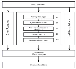
The various stages of identifying the medicinal leaves are explained in detail below. The functional block diagram is given here in Fig. 4.
Grey Image
Quantization
Co-occurrence Matrix
Symmetry
Normalization Leaf Image
Feature Extraction
Classification G
T
S
D
M Local Bin
ar
y P
att
ern
Grey F
eatu
[image:3.595.347.508.590.736.2]res
3.1 Leaf’ statistical features
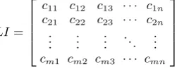
The medicinal leaf image is available as anm×n×ccolour image LI. LI=
c11 c12 c13 · · · c1n c21 c22 c23 · · · c2n
..
. ... ... . .. ... cm1 cm2 cm3 · · · cmn
wherecijrepresents the colour channels of the image. The grey-features using mean, variance, skewness and standard deviation are calculated directly from the original image LI as in Eqns. (2),(3),(4) and (5).
The GTSDM deals only with grey-tone scales and so the given input image LI is converted into am×ngrey-scale image(GI)
GI=
g11 g12 g13 · · · g1n g21 g22 g23 · · · g2n
..
. ... ... . .. ... gm1 gm2 gm3 · · · gmn
wheregijrepresents the grey-tones of the image.
As quantization gives the range of reflectance values in a particular spectral band and the data reduces the radioactive sensitivity of the data, a two-bit image quantization(QI)m×n matrix is obtained
QI=
q11 q12 q13 · · · q1n q21 q22 q23 · · · q2n
..
. ... ... . .. ... qm1 qm2 qm3 · · · qmn
whereqijrepresents the quantized values of the image. The feature computations requires the generation of the co-occurrence matrix from the quantization matrix, which is the GTSDM.
The GTSDM(Mθ) is calculated along the different directions as given in Fig. 2 withθ as0◦,45◦
,90◦ and135◦ with the order k×k. TheMθis in the form
Mθ= fθ
11 f12θ f13θ · · · f1kθ fθ
21 f θ 22 f
θ 23 · · · f
θ 2k ..
. ... ... . .. ... fθ
k1 fk2θ fk3θ · · · fkkθ
wherefθ
ij represents the co-occurences onθdirections of the image.
Here the value of k is determined from the maximum value of the elements ofMθ
i.e. k=max(qij)
where i = 1, 2,· · ·m, and j = 1, 2,· · ·n
The Mθ generated is a square matrix which has dimensions equalling the number of gray levels in the image and the elements correspond to the relative frequencies of the occurrence of pairs of gray level pixels in the image. TheMθis transposed to make the symmetrical matrix(Sθ). The normalized form ofSθisNT
θ, which can be defined as
Sθis normalized to getNθ
Nθ= nθ 11 n θ 12 n θ 13 · · · n
θ 1k nθ
21 nθ22 nθ23 · · · nθ2k .. . ... ... . .. ... nθ k1 n θ k2 n θ k3 · · · n
θ kk
where nθ
ij represents the normalized co-occurences on θ directions.
The second-order statistical features (Fθ
i) are computed from the normalised image(Nθ) for eachθ. The mean feature(MF) vector, as in Eqn.14, is obtained after averaging the feature along all the directions.
MF =1 4
X
θ
X
i
Fiθ (14)
The mean feature values are used for classification in regard to GTSDM features.
The local binary pattern operator also deals with the grey-tone image and the image LI is used to calculate the feature. The local binary pattern operator used 8 neighbours and a unit radius for computation of the pattern. From the computed LBP histogram image as from Eqn. (12) the mean of the histogram is calculated(µL) and used as a feature.
3.2 Feature extraction and classification
Various features from first order statistics, GTSDM feature and LBP are computed. They are mean(µ0), variance(µ2), skewness(µ3), standard deviation(σ), GTSDM Entropy() and LBP mean(µL). Different combinations of the computed features are worked out to find out the best feature combination that will provide the better classification. Initially feature combinations from category C1, C2,...C5 are worked out with few pre-processing filters and then without preprocessing. The texture features are combined into categories as given below. The category combinations chosen are C1(σ•µ3), C2(µ2•µ3), C3(µ0•µ3), C4(µ0•µ3•) and C5(µ0•µ3••µ2•σ•µL). The preprocessing filters that are used with the categories are:
Histogram Equalisation(HE)
Adaptive Histogram Equalisation(AHE)
Contrast Limited Adaptive Histogram Equalisation(CLAHE)
Local Binary Pattern(LBP)
The classification stage has two phases:training and testing. During the training phase, 70% of the dataset samples are used as the training set. The texture features are calculated from the given set of training images and these features are used to train the classifier. During the testing phase, the remaining 30% of the dataset are used as the testing set. The texture features are calculated for the test images and these are the input image to the classifier which finds out the probable plant leaf class category.
4. RESULTS AND DISCUSSION
[image:4.595.107.233.140.189.2]The experimentation has been conducted on medicinal plant leaf database of 5 leaves with 50 sample images in each. Features are computed for each of the 250 medicinal leaf images. The sample feature values computed on images of each leaves are listed in Table 1.
The performance measure for each classifiers are calculated which are presented in tabular and graphical representations. This experiment identified the respective medicinal plant leaves using performance accuracy as the tool.
A sample preprocessed image set consisting of the original image, Histogram equalization image, Adaptive Histogram image, Contrast Limited Adaptive Histogram Equalization image, Local Binary Pattern (LBP) operator image are shown in Fig. 5.
4.1 Preprocessing with category C1
Fig. 5. Processed image sample set
Fig. 6. Classification accuracy with Category C1 on different filters
Fig. 7. Classification accuracy with Category C2 on different filters
accuracy performance values are displayed in the Table 2 and the values are plotted in Fig. 6.
4.2 Preprocessing with category C2
When the preprocessing is done with the category C2, the highest performance obtained for HE is 40% with kNN, for AHE is 38.7% with kNN and for CLAHE is 37.3% with ET and for LBP is 48.0% with SGD and kNN. In this case, LBP with SGD and kNN classification presents 48.0%, which is the best performance. The detailed accuracy performance values are displayed in the Table 3 and the values are plotted in Fig. 7.
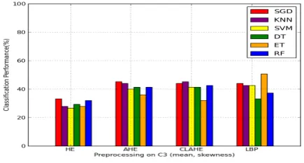
4.3 Preprocessing with category C3
[image:5.595.66.282.255.378.2]When the preprocessing test is carried with the category C3, the best performance obtained for HE is 33.3% with SGD, for AHE is 45.3% with SGD, for CLAHE is 45.3% with kNN and for LBP is 50.7% with ET. In category C3, LBP presents 50.7% with ET classification, which gives the best performance result among the
Fig. 8. Classification accuracy with Category C3 on different filters
Fig. 9. Classification accuracy with Category C4 on different filters
different filters. The detailed accuracy performance values are displayed in the Table 4 and the values are plotted in Fig. 8.
4.4 Preprocessing with category C4
When the preprocessing test is done with the category C4, the best performance obtained for HE is 38.7% with SGD, for AHE and CLAHE is 56% with kNN and for LBP is 44.0% with SGD. In this case, AHE and CLAHE presents 56% with kNN classification, which is the best performance here. The detailed accuracy performance values are displayed in the Table 5 and the values are plotted in Fig. 9.
4.5 Preprocessing with category C5
When the preprocessing test is performed with the category C5, the best result obtained for HE is 57.3% with RF, for AHE is 64% with kNN and CLAHE is 66.7% with kNN and for LBP is 57.3% with kNN. In this case, CLAHE presents 66.7% with kNN classification, which is the best performance. The detailed accuracy performance values are displayed in the Table 6 and the values are plotted in Fig. 10.
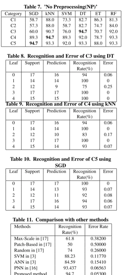
4.6 No Preprocessing(NP)
[image:5.595.323.542.287.412.2] [image:5.595.65.283.427.547.2]Fig. 10. Classification accuracy with Category C5 on different filters
Fig. 11. ’No Preprocessing(NP)’ classification accuracy on different categories
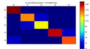
Fig. 12. Confusion matrix of C3 using Decision Tree classifier
[image:6.595.326.527.248.354.2]Fig. 13. Confusion matrix of C4 using kNN classifier
[image:6.595.67.284.309.427.2]Fig. 14. Confusion matrix of C5 using SGD classifier
Fig. 15. Training and Testing possible variation performance for C1
Fig. 16. Training and Testing possible variation performance for C2
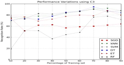
4.7 Training Set Vs Recognition Rate
[image:6.595.325.528.415.522.2] [image:6.595.96.240.504.585.2] [image:6.595.95.240.659.740.2]Fig. 17. Training and Testing possible variation performance for C3
[image:7.595.65.270.261.372.2]Fig. 18. Training and Testing possible variation performance for C4
Fig. 19. Training and Testing possible variation performance for C5
4.8 Performance Analysis
The distribution of the testing set contains 75 of medicinal leaf images(ie. 30% of the dataset) given as support in Fig. 20. The different recognition rate and error rate are calculated as in Eqn.(15) and Eqn.(16) respectively. The recognition rate is the measure of the percentage of the ratio between prediction and the support. They are calculated when the support is having 17 leaf images of leaf 0, 14 leaf images of leaf 1, 12 leaf images of leaf 2, 17 leaf images of leaf 3 and 15 leaf images of leaf 4. The percentages of the leaf images taken for testing is displayed in Fig. 20. The correctly classified leaf images are presented in the prediction.
RecognitionRate= Prediction
Support (15)
Error =1−RecognitionRate (16)
The testing is done 25 times. In this process, the maximum classification performance of 94.7% is obtained though there
Fig. 20. Support for the test images
are some minor deviations in the other performance values. The confusion matrix also have some minor changes in every iterations. Most of the times the result is in the form of the confusion matrix shown in Fig. 12, Fig. 13, and Fig. 14 for categories C3, C4 and C5 respectively.
The decision tree(DT) classifier gives best performance in the No preprocessing C3 category with 100% classification for the medicinal plant leaves, leaf 1, leaf 3 and leaf 4, but the worst performance is produced for leaf 2 with 75 % classification. The detailed recognition rate is shown in Table 8.
The kNN classifier gives best performance in the No processing(NP) C4 category with 100 % classification for the medicinal plant leaves, leaf 1 and leaf 3, but the worst performance is performed for the leaf 2 with 83 % classification. The detailed recognition rate is shown in Table 9.
The SGD classifier gives best performance in the No processing(NP) C5 category with 100 % classification for the medicinal plant leaf, leaf 0 only, but the worst performance is performed for the leaf 2 with 92 % classification. The detailed recognition rate is shown in Table 10.
The error rate is very high for the leaf 2 with 25% in Table 8 , 17% in Table 9, and 8 % in Table 10. The best classification gives very small error rate for the medicinal plant leaf identification. It is necessary to reduce the error rate for better result. The reduction of error rate may depend on the selected features and the dataset.
Much research is done on plant leaf identification. It is imperative to have a further detailed study on the medicinal leaf identification because of it’s importance pertaining to life. Table 11 shows the list of recognition rate of the proposed method and other methods introduced by other researchers. It is shown that the proposed approach gives better recognition rate than the others.
5. CONCLUSION
Herbal medicinal plant leaf identification using texture analyses is a sound method for plant identification. The texture analyses is done using grey textures, GTSDM and lbp texture combinations. The different category combinations using few preprocessing filter and without preprocessing are computed. The method of classifying without preprocessing performed better. The classification performance of 94.7% is obtained using Stochastic Gradient Descent, Decision Tree and kNN classifiers. Therefore it is concluded that the preprocessing approach is not suitable for the medicinal leaf identification. Instead of using preprocessing, the direct application of feature extraction with different categories produced better performance.
[image:7.595.63.271.423.526.2]6. ACKNOWLEGEMENTS
Thanks are due to Dr. J.T.T. KUMARAN, Head, Department of Physics, Nesamony Memorial Christian College, Marthandam, for being a great source of encouragement.
7. REFERENCES
[1] World Health Organization(WHO) Traditional Medicine Fact SheetNo134. Technical report, WHO, Dec 2008. [2] Giuseppe Amato and Fabrizio Falchi. kNN based image
classification relying on local feature similarity. In Proceedings of the Third International Conference on Similarity Search and Applications SISAP ’10, pages 101–108, 2010.
[3] Basavaraj S. Anami, Suvarna S. Nandyal, and A. Govardhan. A combined color, texture and edge features based approach for identification and classification of indian medicinal plants.International Journal of Computer Applications(0975-8887), 6(12):45–51, September 2010. Published By Foundation of Computer Science.
[4] A. Bosch, A. Zisserman, and X. Muoz. Scene classification using a hybrid generative/discriminative approach. IEEE Transactions on Pattern Analysis and Machine Intelligence, 30(4):712 – 727, April 2008.
[5] L. Breiman, J. H. Friedman, R. A. Olshen, and C. J. Stone. Classification and Regression Trees. Chapman Hall, New York, 1984.
[6] Leo Breiman. Random forests.Mach. Learn., 45(1):5–32, October 2001.
[7] Jyotismita Chaki and Ranjan Parekh. Plant leaf recognition using shape based features and neural network classifiers. (IJACSA) International Journal of Advanced Computer Science and Application, 2(10):41–47, 2011.
[8] Jonathan Cheung-Wai Chan and Desir Paelinckx. Evaluation of randomforest and adaboost tree-based ensemble classification and spectral band selection for ecotope mapping using airborne hyperspectral imagery. Remote Sensing of Environment, 112(6):29993011, 16 June 2008. Elsevier.
[9] John Lee Comstock. An introduction to the study of botany: including a treatise on vegetable physiology, and descriptions of the most common plants in the middle and northern states. Robinson, Pratt Co., 1837.
[10] C. Cortes and V. Vapnik. Support-vector networks. Machine Learning, 20:273–297, 1995.
[11] Larry S. Davis and Larry S Davis. Image texture analysis techniques - a survey. InDigital Image Processing, Simon and, pages 189–201, 1980.
[12] Joo Batista Florindo and Odemir Martinez Bruno. Texture classification based on lacunarity descriptor. Image and Signal Processing: Lecture Notes in Computer Science, 7340:513–520, 2012.
[13] Pierre Geurts, Damien Ernst, and Louis Wehenkel. Extremely randomized trees. Machine Learning, 63(1):3–42, 2006.
[14] Robert M. Haralick, K. Shanmugam, and Its’Hak Dinstein. Textural features for image classification. SMC-3(6):610–621, November 1973.
[15] A. Kadir, L. E. Nugroho, A. Susanto, and P. I. Santosa. Neural network application on foliage plant identification. International Journal of Computer Applications, 29(9):15–22, September 2011.
[16] Abdul Kadir, Lukito Edi Nugroho, Adhi Susanto, and Paulus Insap Santosa. Leaf classification using shape, color, and texture features.
[17] Hanife Kebapci, Berrin Yanikoglu, and Gozde Unal. Plant image retrieval using color, shape and texture features.The Computer Journal, 54(9):1475–1490, 2011.
[18] Yuanqing Lin, Fengjun Lv, Shenghuo Zhu, Ming Yang, Timoth´ee Cour, Kai Yu, Liangliang Cao, and Thomas S. Huang. Large-scale image classification: fast feature extraction and svm training. In CVPR’11: IEEE Conference on Computer Vision and Pattern Recognition. [19] Timo Ojala, Matti Pietikinen, and David Harwood. A
comparative study of texture measures with classification based on featured distributions. Pattern recognition, 29(1):51–59, 1996.
[20] Dan C. Popescu, Radu Dobrescu, and Maximillian Nicolae. Texture classification and defect detection using statistical features. International Journal of Circuits, Systems and Signal Processing, 1(1):79–84, 2007.
[21] Subhra Pramanik, Samir Kumar Bandyopadhyay, Debnath Bhattacharyya, and Tai hoon Kim. Identification of plant using leaf image analysis.Springer Signal Processing and Multimedia Communications in Computer and Information Science, 123:291–303, 2010.
[22] S. K. Prof Shah. Image classification based on textural features using artificial neural network (ANN).
[23] Elio Ramos and Denny S. Fernndez;. Classification of leaf epidermis micrographs using texture features. International Journal of Ecoinformatics and Computational Ecology, Ecological Informatics, 4::177–181, 2009.
[24] E. Sandeep Kumar. Leaf color, area and edge features based approach for identification of indian medicinal plants. Indian Journal of Computer Science and Engineering (IJCSE), 3(3):436–442, Jun-Jul 2012.
[25] Junichi Tsujii Tsuruoaka, Yoshimasa and Sophia Ananiadou. Stochastic gradient descent training for l1-regularized log-linear models with cumulative penalty. InACL-IJCNLP 2009, pages 477–485, 2009.
Table 1. Sample Feature Values
Leaf µ0 µ2 µ3 σ µL
0 50.18 663.99 0.58 28.1 5.74 118.98 1 64.48 353.43 -0.47 25.76 5.60 117.80 2 106.71 496.96 -0.24 16.30 3.31 106.68 3 115.52 789.49 -0.01 19.78 2.26 113.03 4 99.46 458.54 -0.02 21.41 3.28 101.83
Table 2. Preprocessing with category C1
Filter SGD kNN SVM DT ET RF HE 33.3 38.7 37.3 29.3 32.0 41.3 AHE 33.3 37.3 24.0 36.0 33.0 41.3 CLAHE 33.3 34.7 24.0 33.3 34.7 38.7 LBP 48.0 49.3 42.7 33.3 34.7 41.3
Table 3. Preprocessing with category C2
Filter SGD kNN SVM DT ET RF HE 32.0 40.0 37.3 29.3 26.7 32.0 AHE 34.7 38.7 24.0 36.0 30.7 37.3 CLAHE 32.0 34.7 25.3 33.3 37.3 34.7 LBP 48.0 48.0 44.0 33.0 36.0 41.3
Table 4. Preprocessing with category C3
Filter SGD kNN SVM DT ET RF HE 33.3 28.0 26.7 29.3 28.0 32.0 AHE 45.3 44.0 40.0 41.3 36.0 41.3 CLAHE 44.0 45.3 41.3 41.3 32.0 42.7 LBP 44.0 42.7 42.7 33.3 50.7 37.3
Table 5. Preprocessing with category C4
Filter SGD kNN SVM DT ET RF HE 38.7 29.3 36.0 36.0 30.7 30.7 AHE 53.3 56.0 38.7 46.7 46.7 41.3 CLAHE 49.3 56.0 40.0 49.3 38.7 52.0 LBP 44.0 42.7 42.7 33.3 38.7 37.3
Table 6. Preprocessing with category C5
[image:9.595.326.533.89.554.2]Filter SGD kNN SVM DT ET RF HE 56.0 46.7 49.3 52.0 46.7 57.3 AHE 52.0 64.0 41.3 53.3 57.3 58.7 CLAHE 56.0 66.7 41.3 60.0 62.7 62.7 LBP 52.0 57.3 46.7 48.0 46.7 56.0
Table 7. ’No Preprocessing(NP)’
Category SGD kNN SVM DT ET RF C1 58.7 88.0 73.3 82.7 86.3 81.3 C2 57.3 88.0 58.7 82.7 74.7 84.0 C3 60.0 90.7 76.0 94.7 70.7 92.0 C4 89.3 94.7 89.3 92.0 78.7 93.3 C5 94.7 93.3 92.0 93.3 88.0 93.3
Table 8. Recognition and Error of C3 using DT
Leaf Support Prediction Recognition Error Rate(%)
0 17 16 94 0.06
1 14 14 100 0
2 12 9 75 0.25
3 17 17 100 0
4 15 15 100 0
Table 9. Recognition and Error of C4 using kNN
Leaf Support Prediction Recognition Error Rate(%)
0 17 16 94 0.06
1 14 14 100 0
2 12 10 83 0.17
3 17 17 100 0
4 15 14 93 0.07
Table 10. Recognition and Error of C5 using SGD
Leaf Support Prediction Recognition Error Rate(%)
0 17 17 100 0
1 14 13 93 0.07
2 12 11 92 0.08
3 17 16 94 0.06
[image:9.595.78.444.89.571.2]4 15 14 93 0.07
Table 11. Comparison with other methods
Methods Recognition Error Rate Rate(%)