An Improved Model for Single Frequency GPS/GALILEO Precise Point Positioning

(1)

http://dx.doi.org/10.4236/pos.2015.62002

An Improved Model for Single-Frequency

GPS/GALILEO Precise Point Positioning

Akram Afifi, Ahmed El-Rabbany

Department of Civil Engineering, Ryerson University, Toronto, Canada Email: akram.afifi@ryerson.ca, rabbany@ryerson.ca

Received 28 April 2015; accepted 25 May 2015; published 28 May 2015

This work is licensed under the Creative Commons Attribution International License (CC BY). http://creativecommons.org/licenses/by/4.0/

Abstract

This paper introduces a new precise point positioning (PPP) model, which combines single-fre- quency GPS/Galileo observations in between-satellite single-difference (BSSD) mode. In the ab-sence of multipath, all receiver-related errors and biases are cancelled out when forming BSSD for a specific constellation. This leaves the satellite originating errors and atmospheric delays un- modelled. Combining GPS and Galileo observables introduces additional biases that have to be modelled, including the GPS to Galileo time offset (GGTO) and the inter-system bias. This paper models all PPP errors rigorously to improve the single-frequency GPS/Galileo PPP solution. GPSPace PPP software of Natural Resources Canada (NRCan) is modified to enable a GPS/Galileo PPP solution and to handle the newly introduced biases. A total of 12 data sets representing the GPS/Galileo measurements of six IGS-MEGX stations are processed to verify the newly developed PPP model. Precise satellite orbit and clock corrections from IGS-MEGX networks are used for both GPS and Galileo measurements. It is shown that sub-decimeter level accuracy is possible with single-frequency GPS/Galileo PPP. In addition, the PPP solution convergence time is improved from approximately 100 minutes for the un-differenced single-frequency GPS/Galileo solution to approximately 65 minutes for the BSSD counterpart when a single reference satellite is used. Moreover, an improvement in the PPP solution convergence time of 35% and 15% is obtained when one and two reference satellites are used, respectively.

Keywords

PPP, GPS, Galileo, BSSD

1. Introduction

(2)

achieved through rigorous modeling or estimation of all errors and biases. Both un-differenced and between- satellite single difference (BSSD) ionosphere-free linear combinations of carrier-phase and pseudorange mea-surements have been used [2] [3]. More recently, [4] showed that a 50% improvement in the PPP convergence time is possible with BSSD dual frequency ionosphere-free GPS, in comparison with the un-differenced coun-terpart. Unfortunately, dual-frequency GPS receivers may not provide a cost-effective solution to many users. In addition, a drawback of a single GNSS system such as GPS is the availability of a sufficient number of visible satellites in urban areas.

The Galileo satellite system offers additional visible satellites to the user, which is expected to enhance the satellite geometry and the overall PPP solution when combined with GPS [5]. As shown in [6], combining GPS and Galileo observations in a PPP solution reduces the convergence time by up to 30% in comparison with the GPS-only PPP solution. Combining GPS and Galileo, however, comes at the expense of introducing additional biases to the observation mathematical models. These include the GPS to Galileo time offset, and Galileo satel-lite hardware delay. Recently, the European Space Agency (ESA) estimated the GPS to Galileo time offset (GGTO), which was found to be approximately 50 ns, or equivalently 15 m range error [7].

Generally, combining multi-constellation observations in a PPP solution improves the positioning accuracy, especially when the system biases are calibrated, as shown in [8]. [9] showed that prior correction of the diffe-rential GPS/Galileo (GIOVE) inter-system biases significantly increases the success rate of instantaneous ambi-guity resolution for short baselines. Likewise, [10] showed that combining GPS/Galileo observables in a double- differenced carrier-phase and pseudorange technique improves the success rate of instantaneous ambiguity res-olution in comparison with GPS-only sres-olution. Unfortunately, however, their work was limited to differential positioning mode.

This paper introduces a new PPP model, which combines single-frequency GPS and Galileo observables in BSSD mode. Precise corrections from the International GNSS Service multi-GNSS experiment (IGS-MEGX) network are used to account for GPS and Galileo satellite orbit and clock errors [11]. As these products are pre-sently referenced to the GPS time and since we use mixed GNSS receivers that also use GPS time as a reference, the GGTO is cancelled out in our model. The inter-system bias is either cancelled out through differencing the observations or is treated as an additional unknown parameter as detailed below. The ionospheric delay is large-ly corrected through the global ionosphere maps (GIM) model [12]. The hydrostatic component of the tropos-pheric zenith path delay is modelled through the Hopfield model, while the wet component is considered as an additional unknown parameter [5]. All remaining errors and biases are accounted for using existing models as shown in [13]. When forming BSSD, we consider three scenarios in the selection of the reference satellite. Ei-ther a GPS or a Galileo satellite is selected as a reference for both GPS and Galileo observables. Alternatively, two reference satellites are selected: a GPS reference satellite for the GPS observables and a Galileo satellite for the Galileo observables. The first approach is sometimes referred to as tight combination, while the latter is sometimes referred to as per constellation or loose combination [9] [14]. It is shown that the use of a single ref-erence satellite provides a sub-decimeter level positioning accuracy and 35% improvement in the convergence time, in comparison with the un-differenced single-frequency GPS/Galileo solution. The use of two reference satellites, although provides comparable positioning accuracy, improves the solution convergence time by 15% only.

2. Un-Differenced GPS/Galileo Model

GNSS observations are affected by random and systematic errors, which must be accounted for to ensure that precise positioning solution is obtained. The positioning accuracy of a PPP model depends on the ability to mitigate errors and biases. These errors can be categorized into three classes, namely satellite related errors, signal propagation related errors, and receiver/antenna associated errors. The main GNSS errors include the sat-ellite/receiver clock errors, satsat-ellite/receiver hardware delays, ionospheric and tropospheric delays, and multi-path [15].

(3)

re-spect to the international atomic time (TAI) [5]. Taking the above errors and biases into consideration and as-suming that the observations are taking simultaneously from a mixed GNSS receiver, which uses GPS time as a reference, the GPS and Galileo observation equations can be written as:

( )

(

,

)

( )

S

(

)

( )

S

(

)

G G G G G G rG G G G G rG G G G G

G G PG

P t t t c d t d t c dt t dt t

T I

ρ τ τ τ

ε

   

= − + _ + − _+ _ − − _

+ + + (1)

( )

(

,

)

( )

S

(

)

( )

S

(

)

E G E G G E rE G E G E rG G E G E

E E PE

P t t t c d t d t c dt t GGTO dt t

T I

ρ τ τ τ

ε

   

= − + _ + − _+ _ − − − _

+ + + (2)

( )

(

)

( )

(

)

( )

(

)

( )

0

( )

0

, S S

G G G G G G rG G G G G rG G G G G

S

G G G r _G G

t t t c t t c dt t dt t

T I N t t

ρ τ δ δ τ τ

λ ϕ ϕ εΦ

   

Φ = − + _ + − _+ _ − − _

 

+ − + _ + − _ + (3)

( )

(

)

( )

(

)

( )

(

)

( )

0

( )

0

, S S

E G E G G E rE G E G E rG G E G E

S

E E E r _E E

t t t c t t c dt t GGTO dt t

T I N t t

ρ τ δ δ τ τ

λ ϕ ϕ εΦ

   

Φ = − + _ + − _+ _ − − − _

 

+ − + _ + − _ + (4)

where, the subscript G refers to the GPS satellite system and the subscript E refers to the Galileo satellite system;

tG is the true signal reception time; τG and τE are signal propagation times for both GPS and Galileo, respectively;

PG and PE are the GPS and Galileo pseudorange measurements, respectively; ΦG and ΦE are the GPS and

Gali-leo carrier-phase measurements, respectively; ρG

(

t tG, G−τG

)

and ρE

(

t tG,G−τE

)

are the GPS and Galileo geometric ranges from the receiver at reception time tG to the satellite at transmission times

(

tG−τG

)

and

(

tG−τE

)

, respectively; dtrG(tG) is the receiver clock error at reception time tG;

(

)

S

G G G

dt t −τ and S

(

)

E G E

dt t −τ are the GPS and Galileo satellite clock errors at transmission times

(

tG−τG

)

and

(

tG−τE

)

, respectively;

drG(tG) and drE(tG) are frequency-dependent code hardware delays in the receiver at reception time tG for GPS and Galileo, respectively; S

(

)

G G G

d t −τ and S

(

)

E G E

d t −τ are frequency-dependent code hardware delays in the satellites at transmission time

(

tG−τG

)

and

(

tG−τE

)

for GPS and Galileo, respectively; δrG(tG) and

(

)

S

G tG G

δ −τ are frequency-dependent carrier phase hardware delays in the receiver at reception time tG for GPS and Galileo, respectively; δrE(tG) and S

(

)

E tG E

δ −τ are frequency-dependent carrier phase hardware delays in the satellites at transmission time

(

tG−τG

)

and

(

tG−τE

)

for GPS and Galileo, respectively; T is the tropos-pheric delay; I is the ionospheric delay; λG and λE are the wavelengths of carrier frequencies for GPS and Galileo signals, respectively; Φr(t0), Φs(t0) are frequency-dependent initial fractional phases in the receiver and satellite channels, respectively; t0 is the receiver (or satellite) initial time; NG and NE are the integer numbers of cycles for GPS and Galileo carrier phase measurements, respectively; GGTO is the GPS to Galileo time offset; c is the speed of light in vacuum; and εP, εΦ are the relevant noise and unmodeled errors.

As indicated earlier, precise orbit and satellite clock corrections of IGS-MGEX network are used for both GPS and Galileo observations. Clock corrections from the two networks are referred to the GPS time. In addi-tion, they include the ionosphere-free linear combination of the satellite hardware delays of L1/L2 P(Y) code for GPS and the ionosphere-free linear combination of the satellite hardware delays of E1/E5a pilot code for Galileo

[16]. As such, using Equations (1)-(4) and dropping the time arguments, the L1/E1 single-frequency code and carrier phase observation equations take the form:

( )

1 1- 2 1

s s

P G rG precG G P P G P PG

P =ρ +dt −c dt_ +β DCB _+T +I +ε (5)

( )

1 1- 2 1- 1 1

s s s

C G rG prec G G P P P C G PG

P =ρ +dt −c dt_ +β DCB +DCB _+T + +I ε (6)

( )

1 1- 5 1

s s

E E rG prec E E E E a E PE

P =ρ +dt −c dt_ +β DCB _+T + +I ISB+ε (7)

( ) 1- 2

1 P P 1 1 1

s s

L ρG dtrG c dt prec G βGDCB  TG I NL εΦL

(4)

( ) 1- 5

1 E E a 1 1 1

s s

E ρE dtrG c dt prec E βEDCB  TE I ISB NE εΦE

Φ = +  − _ + _+ − + +  + (9)

where dts_{prec G}_{( )} and dtsprec E_{( )} are the precise satellites clock corrections for both GPS and Galileo satellites, re-spectively, which are obtained from IGS-MGEX; 1- 2

s P P

DCB , 1- 5

s E E a

DCB and 1- 1 s P C

DCB are the satellite diffe-rential code biases for GPS P1/P2, P1/C1 and Galileo E1/E5a signals, respectively, which are obtained from IGS;

βG and βE are the ionosphere-free linear combination coefficients, which equal 1.546 and 1.261 for GPS and Ga-lileo, respectively; dtrG represents the combined effect of the receiver clock error and the GPS receiver code hardware delay, i.e., dtrG =c d

[

rP1+dtrG

]

when P-code is used and dtrG =c d

[

rC1+dtrG

]

when C/A-code is

used; ISB is the inter-system bias, which equals c d

[

rP1−drE1

]

when P-code is used and equals c d

[

rC1−drE1

]

when C/A-code is used; N is the ambiguity parameter lumped to the satellite and receiver hardware delays,

i.e.,

1 1 1 1 1

S s s

L r rL L rP P

G

N =λ_N+ϕ ϕ− _ +c_δ +δ _−c d_ +d _ (10)

1 1 1 1 1

S s s

E r _E rE E rE E

N =λ_N+ϕ ϕ− _ +c_δ +δ _−c d_ +d _ (11)

It should be pointed out that in both of our GPS-only and GPS/Galileo PPP models, the GPS receiver hard-ware delay is lumped to the receiver clock error as explained above. This strategy maintains the consistency of the estimated receiver clock error for both of the GPS-only and the GPS/Galileo PPP solutions [17]. It should also be mentioned that some of our data sets contain the C/A-code pseudorange rather than the P-code pseudo-range. In this case, Equation (6) should replace Equation (5) for the GPS code measurements. In addition, the receiver clock error would be lumped to the receiver hardware delay of the C/A code. Furthermore, the ISB

would equal the difference in the receiver hardware delays of the C/A code and E1 code, scaled by the speed of light.

Equations (5) to (9) can be simplified for the pseudorange and carrier phase observables after applying the corrections for the satellite clock errors, the hydrostatic component of the tropospheric zenith path delay, the correction to the ionospheric delay, the satellite differential code biases, and the other remaining biases. As stated earlier, the global ionosphere maps (GIM) are used to account for the ionospheric delay [12]. Generally, GIM ionospheric model was found superior to other global models such as the Klobuchar model [18]-[20]. The Hopfield tropospheric correction model is used, along with Vienna mapping function, to account for the hydros-tatic component of the tropospheric delay [21] [22]. All other remaining biases are modeled using existing mod-els, including the effects of ocean loading [23] [24], Earth tide [13], carrier-phase windup [25] [26], Sagnac [27], relativity [5], and satellite and receiver antenna phase-center variations [28]. Applying these corrections and considering P-code observations only lead to:

1 0

G dt m zpd rG f w PG PP

ρ +  + +ε −  = (12)

1 0

E dt m zpdrG f w ISB PE PE

ρ +  + + +ε −  = (13)

1 1 1 0

G dtrG m zpdf w NL L L

ρ +  + +  +ε_Φ − Φ = (14)

1 1 1 0

E dtrG m zpdf w ISB NE E E

ρ +  + + +  +ε_Φ − Φ = (15)

where P and Φ are the corrected carrier phase and pseudorange observables; zpdw is the wet component of the tropospheric zenith path; m_f is the troposphere mapping function; εPG, εPE, εΦL1 and εΦE1 are the noise terms.

3. BSSD GPS/

Galileo Combination Model

(5)

respect to the observations of that satellite. As indicated earlier, this approach is sometimes referred to as tight combination. Alternatively, two reference satellites can be used, i.e., per constellation BSSD. The former ap-proach produces two additional BSSD equations in comparison with the second apap-proach, one for code and another for carrier-phase observables. However, the ISB is cancelled out when the per-constellation approach is used. When a GPS satellite is used as a reference in a tight combination, we obtain:

, 1 0

ij ij ij ij

G G m zpdf w PG PP

ρ ε

∇ + + ∇ − ∇ = (16)

, 1 0

ik ik ik ik

E G m zpdf w ISB PPE E G

ρ ε

∇ + + + ∇ − ∇ = (17)

, 1 1 1 0

ij ij ij ij ij

G G m zpdf w NL L L

ρ εΦ

∇ + +  + ∇ − ∇Φ = (18)

, 1 1 1 0

ik ik ik ik ik

E G m zpdf w ISB NE E E G

ρ ε_Φ

∇ + + +  + ∇ − ∇Φ = (19)

where ∇ refers to the BSSD operator; 1 ij L

N and 1 ik E

N are the BSSD non-integer the ambiguity parameters lumped to the receiver and satellite hardware delays as shown in Equations (20) and (21).

1 1 1 1 1

ij j i j i j i j i

L G G G G L L P P

N =λ_N −N _−λ ϕ_ −ϕ _+c_δ −δ _−c d_ −d _ (20)

1 1 1 1 1

1 1 1 1

ik k i i k k i

E E G G E rE E rL L

k i

rE E rP P

N N N c c

c d d c d d

λ  λ ϕ ϕ  δ δ  δ δ 

= _ − _− _ − _+ _ + _− _ + _

   

− _ + _+ _ + _



(21)

If, however, a Galileo satellite is used as a reference in a tight combination, we obtain the following set of BSSD equations:

, 1 0

lj lj lj lj

G E m zpdf w ISB PG PP E

ρ ε

∇ + − + ∇ − ∇ = (22)

, 1 0

lk lk lk lk

E E m zpdf w PE P E

ρ ε

∇ + + ∇ − ∇ = (23)

, 1 1 1 0

lj lj lj lj lj

G E m zpdf w ISB NL L L E

ρ εΦ

∇ + − +  + ∇ − ∇Φ = (24)

, 1 1 1 0

lk lk lk lk lk

E E m zpdf w NE E E

ρ εΦ

∇ + +  + ∇ − ∇Φ = (25)

where, 1 lj L

N and 1 lk E

N are the BSSD non-integer ambiguity parameters lumped to the receiver and satellite hardware delays as shown in Equations (26) and (27).

1 1 1 1 1

1 1 1 1

lj j l l j j l

L G E E G rL L rE E

j l

rP P rE E

N N N c c

c d d c d d

λ  λ ϕ ϕ  δ δ  δ δ 

= _ − _− _ − _+ _ + _− _ + _

   

− _ + _+ _ + _



(26)

1 1 1 1 1

lk k l k l k l k l

E E E E E E E E E

N =λ_N −N _−λ ϕ_ −ϕ _+c_δ −δ _−c d_ −d _ (27)

Finally, the per-constellation BSSD equations take the form:

, 1 0

ij ij ij ij

G G m zpdf w PG PP

ρ ε

∇ + + ∇ − ∇ = (28)

, 1 0

lk lk lk lk

E E m zpdf w PE P E

ρ ε

∇ + + ∇ − ∇ = (29)

, 1 1 1 0

ij ij ij ij ij

G G m zpdf w NL L L

ρ εΦ

∇ + +  + ∇ − ∇Φ = (30)

, 1 1 1 0

lk lk lk lk lk

E E m zpdf w NE E E

ρ ε_Φ

∇ + +  + ∇ − ∇Φ = (31)

where, 1 ij L

N and 1 lk E

(6)

hardware delays as shown in Equations (32) and (33).

1 1 1 1 1

ij j i j i j i j i

L G G G G L L P P

N =λ_N −N _−λ ϕ_ −ϕ _+c_δ −δ _−c d_ −d _ (32)

1 1 1 1 1

lk k l k l k l k l

E E E E E E E E E

N =λ_N −N _−λ ϕ_ −ϕ _+c_δ −δ _−c d_ −d _ (33)

It should be noticed from the above equations that the modified receiver clock error (i.e., the common term

rG

dt ) and the initial phase bias cancel out when forming BSSD with one satellite selected as a reference (i.e., tight combination). However, when forming per constellation BSSD, the modified receiver clock error, the inter- system bias, and the initial phase bias are all cancelled out.

4. S

equential Least Squares Estimation

The sequential least-squares estimation technique is used to obtain the best estimates, in the least squares sense, of the unknown parameters. The noise terms in the above observations equations are modeled stochastically us-ing an exponential function, as described in [6]. They showed that, in comparison with existing stochastic mod-els such as the general sine function, the use of the exponential model improves the PPP solution precision and convergence time. The general linearized form for the above observations equations around the initial (approx-imate) vector u0 and observables 𝑙𝑙 can be written in a compact form as:

( )

, ≈ ∆ − − ≈0

f u l A u w r (34)

where u is the vector of unknown parameters; A is the design matrix, which includes the partial derivatives of the observation equations with respect to the unknown parameters u; Δu is the unknown vector of corrections to the approximate parameters u0, i.e., u = u0 + Δu; w is the misclosure vector and r is the vector of residuals. The sequential least-squares solution for the unknown parameters Δuiat an epoch i can be obtained from (Vanicek

and Krakiwsky, 1986):

(

)

1

[

]

1 T 1 T

1 1 i 1 1

i i i i l i i i i i i

−

− −

− − − −

∆ = ∆u u +M A C +A M A w − ∆A u (35)

(

)

1

1 1 1 T 1 T 1 1 1 i 1 1

i i i i l i i i i

−

− − − − −

− − − −

= − +

M M M A C A M A A M (36)

(

)

1

-1 1 1 T 1 T 1

1 1 1 1

i i

u i i i i l i i i i

−

− − − −

∆ = = − − − + − −

C M M M A C A M A A M (37)

where Δui−1 is the least-squares solution for the estimated parameters at epoch i − 1; M is the matrix of the nor-mal equations; Cl and CΔu are the covariance matrices of the observations and unknown parameters, respectively. It should be pointed out that the usual batch least-squares adjustment should be used in the first epoch, i.e., for i

= 1. The batch solution for the estimated parameters and the inverse of the normal equation matrix are given re-spectively by [29]:

0 ₁ ₁

1 1 T 1 T 1 1 _x 1 l 1 1 l 1

−

− − −

 

∆ =u _C +A C A_ A C w (38)

0 ₁

1 1 1 T 1 1 _x 1 l 1

− − ₌_ − ₊ − _

 

M C A C A (39)

where Cx0 is a priori covariance matrix for the approximate values of the unknown parameters.

Under the assumption that the observations are uncorrelated and the errors are normally distributed with zero mean, the covariance matrix of the un-differenced observations takes the form of a diagonal matrix. The ele-ments along the diagonal line represent the variances of the code and carrier phase measureele-ments. In our solu-tion, we consider that the ration between the standard deviation of the code and carrier-phase measurements to be 100. When forming BSSD, however, the differenced observations become mathematically correlated. This leads to a fully populated covariance matrix at a particular epoch.

(7)

1 1 1

1

0 0 0

1 1 1

0 0 0

1 1 1

1

0 0 0

1 1 1

0 0 0

0

1 0 0 0 0 0

1 0 1 0 0 0

1 0 0 0 0 0

G G G

G

G G G

G

G G G

G

G G G

G

f

n n n

n f

n n n

n

x X y Y z Z

m

x X y Y z Z

m

x X y Y z Z

m

x X

ρ ρ ρ

 −   −   −               −   −   −               −   −   −              − = A                   0 0

0 0 0

1 1

1

0 0 0

1 1 0 0 1 0 1 1 1

0 0 0

1 1

1

0 0 0

0

1 0 0 1 0 0

1 1 0 0 0 0

1 1 0 0 1 0

G G

G

G G G

E E E

E

E E E

E

E E E

E

n n

n f

n n n

f

n n

y Y z Z

m

x X y Y z Z

m

x X y Y z Z

m

x X

ρ ρ ρ

ρ    −   −               −   −   −               −   −   −               −                       ( ) 1 1 0 0 0 0

0 0 0

0 0 0 ₂ ₆

1 1 0 0 0 0

1 1 0 0 0 1

E E

E

E E E

E

E E E

r G w L n n n f n n

n n n

n f

n n n

n n x y z dt zpd ISB N N

y Y z Z

m

x X y Y z Z

m

ρ ρ

ρ ρ ρ _{× +}

            ∆     _∆     ∆           _{∆ =}                    _ ₋ _{ } ₋ _          _ _{ } _     −   −   −          _ _{ } _{ } _    u         1 1 1 1 6 G E n L E n E n N N ₊                                          (40)

where nG refers to the number of visible GPS satellites; nE refers to the number of visible Galileo satellites;

G E

n=n +n is the total number of the observed satellites for both GPS and Galileo systems; x0, y0 and z0 are the approximate receiver coordinates; jG, jG, jG, 1, 2, ,

G

X Y Z j=  n are the known GPS satellite coordinates; , , , 1, 2, ,

E E E

k k k

E

X Y Z k=  n are the known Galileo satellite coordinates; ρ0 is the approximate receiver- satellite range. The unknown parameters in the above system are the corrections to the receiver coordinates, Δx, Δy, and Δz, the biased receiver clock error dtr_G, the wet component of the tropospheric zenith path delay zpdw, the inter-system bias ISB, and the non-integer ambiguity parameters N . It should be pointed out that the num-ber of unknown parameters in the above system equals nG+nE+6, while the number of equations equals

2nG+2nE. This means that the redundancy equals nG+nE−6. In other words, at least 6 mixed satellites are needed for the solution to exist. In comparison with the GPS-only un-differenced scenario, which requires a minimum of 5 satellites for the solution to exist, the addition of Galileo satellites increases the redundancy by nE − 1. In other words, we need a minimum of two Galileo satellites in order to contribute to the solution.

When a GPS satellite is selected as a reference to form the BSSD for both GPS and Galileo observations, the design matrix A and the vector of corrections Δu take the form:

2 2 2

1 1 1

2 1

0 0 0 0 0 0

1 1 1

0 0 0 0 0 0

1 1

0 0 0 0 0 0

1 1

0 0 0 0 0

2 2 2

0 0 0 0 0

G G G G G G

G G

G G G G G G

G G G G G

f

x X x X y Y y Y z Z z Z

m

x X x X y Y y Y z Z z

ρ ρ ρ ρ ρ ρ

ρ ρ ρ ρ ρ

 −  ₋ −   −  ₋ −   −  ₋ −                           −  ₋ −   −  ₋ −   − ₋ −                     = A   1 2 1 1 0

1 1 1

1

0 0 0 0 0 0

1 1 1

0 0 0 0 0 0

1

0 0 0

1

0 0 0

0 1 0 0 0

0 0 0 0 0

G G G

G

G G G G G G

G G

G G G G G G

G G G

f

n n n

n f

n n n

n n

Z m

m

x X x X y Y y

ρ

ρ ρ ρ ρ ρ ρ

ρ ρ ρ

       −  ₋ −   −  ₋ −   −  ₋ −                           −  ₋ −   − ₋                            1 1 1

0 0 0

1 1

0 0 0

1 1 1

1 1

0 0 0 0 0 0

1 1 1 1 1

0 0 0 0 0 0

1 1 0 0 1 1 1 1 0 0

0 0 1 0 0

1 0 0 0 0

G G G

G G

G G G

E E E

E G

E G E G E G

G E E G n n f n f

Y z Z z Z

m

x X x X

ρ ρ ρ

ρ ρ ρ ρ ρ ρ

ρ ρ  −   −  ₋ −                     − ₋ −  − ₋ −  − ₋ −                          − ₋ −        

1 1 1

1 1

0 0 0 0

1 1 1

0 0 0 0

1 1 1

1

0 0 0 0 0 0

1 1 1

0 0 0

1 1

0

0 0

1 0 0 1 0

1 0

G G

E E

E G

E G E G

G G G

E E E

E G

G G G

f

n n n

n f

n n n

y Y y Y z Z z Z m

m

ρ ρ ρ ρ

ρ ρ ρ ρ ρ ρ

   − ₋ −   − ₋ −                             −  −  −  −  −  − −  −  −                                 ( ) ( )

1 1 1

1

0 0 0 0 0 0

1 1 1

0 0 0 0 0 0 2 1 4

0 0 0

1 0 0 0 1

G G G

E E E

E G

E G E G E G

w

n n n

n f

n n n

n n

x y z zpd

m

ρ ρ ρ ρ ρ ρ _{− × +}

(8)

where 1G refers to the GPS reference satellite. All other parameters are as defined above. The advantage of the above system (42) is that the number of unknown parameters is reduced by two (i.e., becomes nG+nE+4), in comparison with the un-differenced scenario. This, however, comes at the expense of reducing the number of BSSD observation equations to 2

(

nG+nE−1

)

. As such, the redundancy remains unchanged and equals

6

G E

n +n − . Similarly, we need a minimum of two Galileo satellites in order to contribute to the solution. By analogy, the use of a Galileo satellite as a reference to form the BSSD for both GPS and Galileo observations leads to:

1 1 1

1 1

1 1 1

0 0 0 0 0 0

1 1 1

0

0 0 0 0 0

1 1

0 0 0 0

1 1

0 0

1 1

0

0 0 0 0

1

1 0 0 0 0

G G E G E

E

G G G G G

G G E G

G G G G

E G E E E f

m

x X x X y Y y Y z Z z

ρ

ρ ρ ρ ρ ρ

ρ

ρ ρ ρ ρ

 − ₋ −   −  ₋ −   −  ₋ −                           − ₋ −   −  ₋ −   − ₋ −                     = A   1 1 0

1 1 1

1

0 0 0 0 0 0

1 1 1

0 0 0 0 0 0

1

0 0 0

1

0 0 0

1 1

1 1 0 0 0

1 0 0 0 0

E E

G

G E G E G E

G E

G G G G G G

G E G

G G

G

f

n n n

n f

n n n

n n

Z m

m

x X x X y Y y

ρ

ρ ρ ρ ρ ρ ρ

ρ ρ ρ

       −  ₋ −   −  ₋ −   −  ₋ −                           −  ₋ −   − ₋                            1 2 1 1 1 1

0 0 0

1 1

0 0 0

1 1 1 1 1

0 0 0 0 0 0

1 1 1 1 1

0 0 0 0 0 0

1 1 0 0 1 1 0 1 0

1 0 1 0 0

0 0 0 0 0

G

E E

G E

G G G

E E E E E E

E

E G E G E G

E E E G E n n f n f

Y z Z z Z

m

x X x X

ρ ρ ρ

ρ ρ ρ ρ ρ ρ

ρ ρ  −   −  ₋ −                     −  −  −  −  −  − −  −  −                     − ₋ −        

1 1 1

0 0 0 0

1 1 1

0 0 0 0

1 1 1

1

0 0 0 0 0 0

1 1 1

0 0 0 0 0 0

1

2 1

1 0 0 0 1 0

0 0

E E E E

E

E G E G

E E E E E E

E E

G E

G G

f

n n n

n f

n n n

y Y y Y z Z z Z m

m

ρ ρ ρ ρ

ρ ρ ρ ρ ρ ρ

   − ₋ −   − ₋ −                             − ₋ −  − ₋ −  − ₋ −                                      ( ) ( )

1 1 1

1

0 0 0 0 0 0

1 1 1

0 0 0 0 0 0 2 1 4

0 0 0

0 0 0 0 1

E E E E E E

E E

E G E G E G

w

n n n

n f

n n n

n n

x y z zpd

m

ρ ρ ρ ρ ρ ρ _{− × +}

              ∆     _∆     ∆         _{∆ =}                                  −  −  −  −  −  −  ₋ ₋ ₋                              u     1 1 1 1 21 1 1 4 1 1 E G E E E E L n L E n E n ISB N N N N ₊                 ∇       ∇   _∇      _∇          (42)

where 1E refers to the Galileo reference satellite. All other parameters are as defined above. Similar to the above BSSD scenario, the redundancy remains unchanged and equals nG +nE−6.

When two reference satellites are selected to form the BSSD, i.e., per-constellation BSSD, the design matrix

A and the vector of corrections Δu take the form:

2 1 2 1 2 1

2 1

0 0 0 0 0 0

1 1

2 1

0 0 0 0 0 0

1 1

0 0 0 0 0 0

1 2 2 2 2 1 0 0 2 2 0 0 2 2 0

0 0 0 0

G G G G G G

G G

G G G G G G

G G G G G

f

m

ρ ρ ρ ρ ρ ρ

ρ ρ ρ ρ ρ

 −  ₋ −   −  ₋ −   −  ₋ −                           −  ₋ −   −  ₋ −   − ₋ −                     = A   1 2 1 1 0

1 1 1

1

0 0 0 0 0 0

1 1 1

0 0 0 0 0 0

1 1

0 0 0 0

1

0 0 0

1 0 0 0

0 0 0 0

G G G

G

G G G G G G

G G

G G G G G G

G G G

f

n n n

n f

n n n

n n

m

x X x X y Y y Y

ρ

ρ ρ ρ ρ ρ ρ

ρ ρ ρ

       −  ₋ −   −  ₋ −   −  ₋ −                           −  ₋ −   − ₋ −                           1 1 1 1 0 0 1 1

0 0 0

1 1 1 1 1

2 1

0 0 0 0 0 0

1 1 1 1 1

0 0 0 0 0 0

1 1

0 0

1 1

0 0

0 1 0 0

0 0 0 0

G G G

G G

G G G

E E E E E E

E E

E G E G E G

E E E G n n f n f

z Z z Z

m

x X x X

ρ ρ ρ

ρ ρ ρ ρ ρ ρ

ρ ρ    −  ₋ −                     − ₋ −  − ₋ −  − ₋ −                            −  − −            

1 1 1

2 1

0 0 0 0

1 1 1

0 0 0 0

1 1 1

1

0 0 0 0 0 0

1 1 1

0 0 0 0 0

1

0

1 0 0 1 0

0 0 0 0

E E E E

E E

E G E G

E E E E E E

E E

G G G

f

n n n

n f

n n n

y Y y Y z Z z Z

m

x X

ρ ρ ρ ρ

ρ ρ ρ ρ ρ ρ

     −  −  −  − −  −                     − ₋ −  − ₋ −  − ₋ −                         −               ( ) ( ) 21 1

1 1 1

1

0 0 0 0 0

1 1 1

0 0 0 0 0 0 ₂ ₂ ₂

0 0 0 1

G

E E E E E E

E E

E G E G E G

w L

n n n

n f

n n n

n n x y z zpd N

x X y Y y Y z Z z Z

m

ρ ρ ρ ρ ρ ρ

− × +                 _∆     ∆   ∆       ∇   ∆ =       ∇                             −  −  −  −  −  ₋ ₋ ₋                              u     1 1 12 1 1 1 2 G G E E E n L E n E n N N N ₊                       ∇       ∇        (43)

(9)

that the redundancy remains unchanged and equals nG+nE−6. Similar to the previous scenarios, the redun-dancy for the GPS-only scenario is still nG−5 and the addition of Galileo satellites increased the overall re-dundancy to nE−1. As such, we still need a minimum of two Galileo satellites in order to contribute to the so-lution. However, as indicated by [14], the adjustment model is stronger through the tight combination, i.e., when a single satellite is used as a reference.

5. Results and Discussion

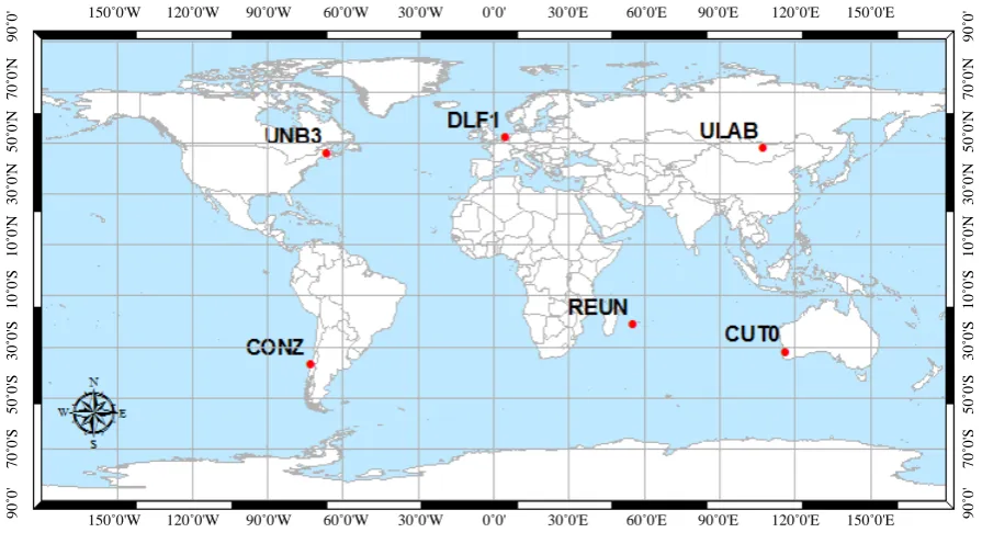
To verify the developed GPS/Galileo PPP model, GPS and Galileo measurements at six well-distributed stations

(Figure 1) were selected from the IGS tracking network [28]. Those stations are occupied by GNSS receivers,

which are capable of simultaneously tracking the GPS and Galileo constellations. The analysis is performed on two different days January 1, 2014 and July 8, 2014 for all stations shown in Figure 1.

The sampling interval for all data sets is 30 seconds, while the time span used in the analysis is three hours, which is selected at different times of the day to ensure that the four Galileo satellites are visible at each station. GPSPace PPP software of Natural Resources Canada (NRCan) was modified to enable a GPS/Galileo PPP solu-tion as described above. The posisolu-tioning results for stasolu-tions CONZ, and CUT0 (January 1, 2014) and stasolu-tions DLF1, and UNB3 (July 8, 2014) are presented below. Similar results are obtained from the other stations. How-ever, a summary of the convergence times is presented below for all stations.

The single-frequency GPS/Galileo PPP solution is implemented through combining the GPS L1 signal with the Galileo E1 signal. As mentioned earlier, three different scenarios are considered when processing the data sets with the BSSD model, namely (1) a GPS satellite is selected as a reference satellite for both GPS and Gali-leo observables; (2) a GaliGali-leo satellite is selected as a reference satellite for both GPS and GaliGali-leo observables; and (3) two reference satellites are selected: a GPS reference satellite for the GPS observables and a Galileo sa-tellite for the Galileo observables. To assess the PPP solution accuracy of the developed single-frequency model, un-differenced dual-frequency ionosphere-free linear combination of GPS/Galileo PPP is used as a reference.

Figure 2 shows the reference solution for July 8, 2014, as an example. As can be seen, the dual-frequency

[image:9.595.89.537.462.710.2]

GPS/Galileo PPP solution has a sub-decimeter positioning accuracy with approximately 15 minutes conver-gence time (i.e., the time that the solution takes to converge to a decimetre-level positioning accuracy).

Figure 3 shows the PPP results for the un-differenced single-frequency GPS/Galileo model. As can be seen,

the single-frequency GPS/Galileo PPP solution shows a decimetre level accuracy and approximately 100 mi-nutes convergence time. It should be emphasized that the exponential function is used to model the stochastic

150˚0'W 120˚0'W 90˚0'W 60˚0'W 30˚0'W 0˚0' 30˚0'E 60˚0'E 90˚0'E 120˚0'E 150˚0'E 150˚0'W 120˚0'W 90˚0'W 60˚0'W 30˚0'W 0˚0' 30˚0'E 60˚0'E 90˚0'E 120˚0'E 150˚0'E

90

˚0'

70

˚0

'S

50

˚0

'S

30

˚0

'S

10

˚0

'S

10

˚0

'N

30

˚0

'N

50

˚0

'N

70

˚0

'N

90

˚0'

90

˚0'

70

˚0

'S

50

˚0

'S

30

˚0

'S

10

˚0

'S

10

˚0

'N

30

˚0

'N

50

˚0

'N

70

˚0

'N

90

˚0'

(10)

Time (min)

ΔE ΔN ΔU DLF1 - July 8, 2014

0 10 20 30 40 50 60

-5 -4 -3 -2 -1 0 1 2 3

E

rr

o

r (m

)

Time (min)

ΔE ΔN ΔU UNB3 - July 8, 2014

0 10 20 30 40 50 60

-4 -3 -2 -1 0 1 2 3

E

rr

o

r (m

[image:10.595.75.540.75.402.2]

)

Figure 2.Un-differenced ionosphere-free GPS/Galileo PPP solution.

Time (min)

0 20 40 60

-5 -4 -3 -2 -1 0 1 2 3

E

rr

o

r (m

)

80 100 120 140 160 180 4

5

Time (min)

0 20 40 60

-5 -4 -3 -2 -1 0 1 2 3

E

rr

o

r (m

)

80 100 120 140 160 180 4

5

Figure 3. Un-differenced single-frequency GPS/Galileo PPP solution.

part of the mathematical model. As shown in [6], the use of the exponential function improves the precision of the PPP solution by about 30%, in comparison with the sine function.

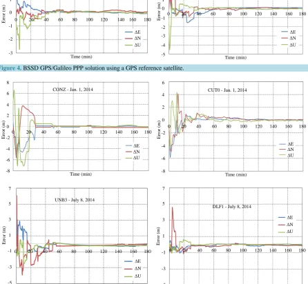
Figure 4 shows the results of the single-frequency BSSD GPS/Galileo PPP model, when a GPS satellite is

selected as a reference for both GPS and Galileo observables. As can be seen, similar to the un-differenced counterpart, a sub-decimeter level positioning accuracy is obtained. However, a reduction of about 35% in the convergence time is obtained through the BSSD model, in comparison with the un-differenced single-frequency GPS/Galileo solution.

Figure 5 shows the results of the BSSD GPS/Galileo PPP solution when a Galileo satellite is selected as a

reference for both GPS and Galileo observables. As expected, similar results to the previous scenario are ob-tained. This similarity is due mainly to the fact that both BSSD models use tight combination with similar rela-tive satellite geometry and same redundancy number.

The results of the third BSSD model scenario, i.e., when a GPS satellite and a Galileo satellite are selected as references for the GPS and Galileo observables, respectively, are shown inFigure 6. As can be seen, similar to the previous two scenarios, a sub-decimeter level positioning accuracy is obtained. However, only a 15% reduc-tion in the convergence time is obtained, in comparison with the un-differenced model solureduc-tion. This moderate improvement in the convergence time is likely attributed to the fact that the loose combination is weaker than the tight combination, as indicated above. In addition, as the ionospheric delay would not be modelled suffi-ciently through the GIM, a residual component remains, which would be mapped differently into the unknown parameters of the BSSD models.

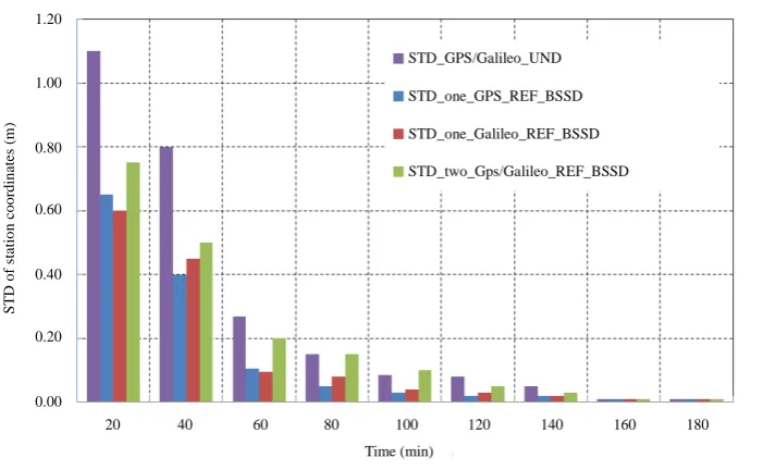
Figure 7shows a summary of the standard deviations (STD) for the obtained station coordinates, which are

[image:10.595.92.536.82.230.2]

(11)

Time (min)

ΔE ΔN ΔU CONZ - Jan. 1, 2014

0 20 40 60

-8 -6 -4 -2 0 2

E

rr

o

r (m

)

80 100 120 140 160 180 4

6

Time (min)

ΔE ΔN ΔU CUT0 - Jan. 1, 2014

0 20 40 60

-8 -6 -4 -2 0 2

E

rr

o

r (m

)

80 100 120 140 160 180 4

6

Time (min)

0 20 40 60 0

E

rr

o

r (m

)

80 100 120 140 160 180 2

3

-3 -2 -1 1

Time (min)

0 20 40 60

-5 0

E

rr

o

r (m

)

80 100 120 140 160 180 2

3 4

[image:11.595.80.540.105.553.2]

-4 -3 -2 -1 1

Figure 4. BSSD GPS/Galileo PPP solution using a GPS reference satellite.

Time (min)

0 20 40 60

-8 -6 -4 0 2

E

rr

o

r (m

)

80 100 120 140 160 180 4

6

-2 8

Time (min)

0 20 40 60

-8 -6 -4 -2 0 2

E

rr

o

r (m

)

80 100 120 140 160 180 4

6

Time (min)

0 20 40 60

-5 -3 -1 1 3

E

rr

o

r (m

)

80 100 120 140 160 180 5

7

Time (min)

0 20 40 60

-5 -3 -1 1 3

E

rr

o

r (m

)

80 100 120 140 160 180 5

7

[image:11.595.90.537.277.689.2]

(12)

Time (min)

0 20 40 60

-8 -6 -4 -2 0 2

E

rr

o

r (m

)

80 100 120 140 160 180 4

6

Time (min)

0 20 40 60

-5 -4 -3 -2 -1

E

rr

o

r (m

)

80 100 120 140 160 180 0

1

Time (min)

0 20 40 60

-8 -6 -4 -2 0 2

E

rr

o

r (m

)

80 100 120 140 160 180 4

6

Time (min)

0 20 40 60

-8 -6 -4 -2 0 2

E

rr

o

r (m

)

80 100 120 140 160 180 4

[image:12.595.81.534.79.360.2]

6

Figure 6. BSSD GPS/Galileo PPP solution using two reference satellites.

Time (min)

STD_GPS/Galileo_UND

20 40 60 0.00

S

T

D

of

s

ta

ti

o

n c

oor

di

na

te

s (

m

)

80 100 120 140 160 180 0.20

0.40 0.60 0.80 1.00 1.20

STD_one_GPS_REF_BSSD

STD_one_Galileo_REF_BSSD

STD_two_Gps/Galileo_REF_BSSD

Figure 7. Summary of standard deviations of obtained station coordinates.

[image:12.595.115.546.130.601.2]

discussed above, this is likely attributed to the relatively weaker adjustment model of the loose combination.

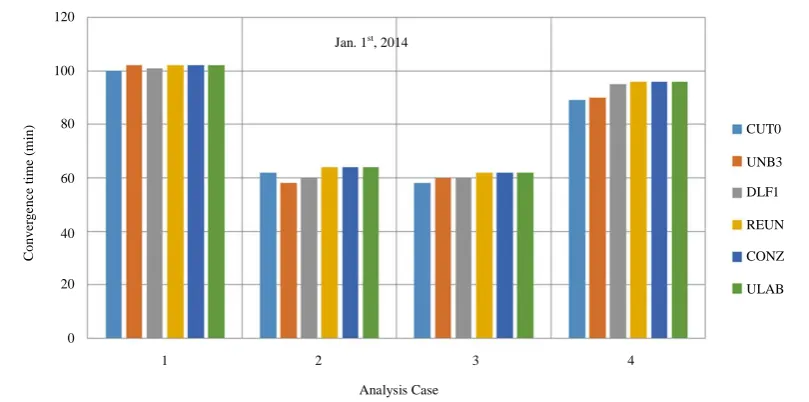
Figure 8 summarizes the convergence times of all 24 cases considered in our analysis. As shown in Figure 9,

as far as the solution convergence time is concerned, the best results are obtained when the BSSD model with one reference satellite (i.e., a tight combination) is used.

[image:12.595.143.494.383.599.2]

(13)

1

C

onve

rge

nc

e t

im

e (

m

in)

2 3 4

Analysis Case 0

20 40 60 80 100 120

Jan. 1st, 2014

ULAB CUT0

UNB3

DLF1

REUN

[image:13.595.106.511.81.282.2]

CONZ

Figure 8. Summary of convergence times for all data sets analysed. (1) Un-differenced model; (2) BSSD

model with a GPS satellite as a reference; (3) BSSD model with a Galileo satellite as a reference; (4) BSSD model with both a GPS and a Galileo as reference satellites.

Time (min) 20 40 60

0

IS

B

(

m

)

80 100 120 140 160 180 0

3 6 9 12 15 18

REUN ULAB CONZ UNB3 DLF1

CUT0

Figure 9.Summary of ISB results.

As shown in Figure 9, the values of the ISB are stable over the observation time spans. Differences of up to 3 m can be observed, which indicate that the ISB is receiver/firmware dependent.

6. Conclusions

[image:13.595.118.507.328.528.2]

(14)

The values of the ISB have been obtained for various days and receiver types. Almost identical results have been obtained with both of the un-differenced and BSSD (tight combination) modes. It has been found that the values of the ISB are largely stable over the observation time spans. However, differences of up to 3 m have been observed, which suggest that the ISB is receiver/firmware dependent.

Acknowledgements

This research was partially supported by the Natural Sciences and Engineering Research Council (NSERC) of Canada, the Government of Ontario, and Ryerson University. The authors would like to thank the International GNSS service (IGS) network for providing the satellites precise products.

References

[1] Zumberge, J.F., Heflin, M.B., Jefferson, D.C., Watkins, M.M. and Webb, F.H. (1997) Precise Point Processing for the Efficient and Robust Analysis of GPS Data from Large Networks. Journal of Geophysical Research, 102, 5005-5017.

http://dx.doi.org/10.1029/96JB03860

[2] Heroux, P. and Kouba, J. (2001) GPS Precise Point Positioning Using IGS Orbit Products. Physics and Chemistry of

the Earth, Part A: Solid Earth and Geodesy, 26, 573-578. http://dx.doi.org/10.1016/S1464-1895(01)00103-X

[3] Colombo, O.L., Sutter, A.W. and Evans, A.G. (2004) Evaluation of Precise, Kinematic GPS Point Positioning. ION

GNSS 17th International Technical Meeting of the Satellite Division, 21-24 September 2004, Long Beach.

[4] Elsobeiey, M. and El-Rabbany, A. (2014) Efficient Between-Satellite Single-Difference Precise Point Positioning Model. Journal of Surveying Engineering, 140, Article ID: 04014007.

http://dx.doi.org/10.1016/S1464-1895(01)00103-X

[5] Hofmann-Wellenhof, B., Lichtenegger, H. and Wasle, E. (2008) GNSS Global Navigation Satellite Systems: GPS, Glonass, Galileo & More. Springer Wien, New York, 501 p.

[6] Afifi, A. and El-Rabbany, A. (2013) Stochastic Modeling of Galileo E1 and E5a Signals. International Journal of

En-gineering and Innovative Technology (IJEIT), 3, 188-192.

[7] European Space Agency (ESA) (2013) Galileo and GPS Synchronise Watches: New Time Offset Helps Working To-gether.

http://www.esa.int/Our_Activities/Navigation/Galileo_and_GPS_synchronise_watches_new_time_offset_helps_worki ng_together

[8] Melgard, T., Tegedor, J., de Jong, K., Lapucha, D. and Lachapelle, G. (2013) Interchangeable Integration of GPS and Galileo by Using a Common System Clock in PPP. ION GNSS+, 16-20 September 2013, Institute of Navigation, Nashville.

[9] Odijk, D. and Teunissen, P.J.G. (2013) Characterization of Between-Receiver GPS-Galileo Inter-System Biases and Their Effect on Mixed Ambiguity Resolution. GPS Solutions, 17, 521-533.

http://dx.doi.org/10.1007/s10291-012-0298-0

[10] Paziewski, J. and Wielgosz, P. (2013) Assessment of GPS + Galileo and Multi-Frequency Galileo Single-Epoch Pre-cise Positioning with Network Corrections. GPS Solutions, 18, 571-579. http://dx.doi.org/10.1007/s10291-013-0355-3

[11] Montenbruck, O., Steigenberger, P., Khachikyan, R., Weber, G., Langley, R.B., Mervart, L. and Hugentobler, U. (2014) IGS-MGEX: Preparing the Ground for Multi-Constellation GNSS Science. Inside GNSS, 9, 42-49.

[12] Schaer, S., Gurtner, W. and Feltens, J. (1998) IONEX: The IONosphere Map Exchange Format Version 1.

http://igscb.jpl.nasa.gov/igscb/data/format/ionex1.pdf

[13] Kouba, J. (2009) A Guide to Using International GNSS Service (IGS) Products.

http://igscb.jpl.nasa.gov/igscb/resource/pubs/UsingIGSProductsVer21.pdf

[14] Paziewski, J. and Wielgosz, P. (2014) Accounting for Galileo-GPS Inter-System Biases in Precise Satellite Positioning.

Journal of Geodesy, 89, 81-93. http://dx.doi.org/10.1007/s00190-014-0763-3

[15] El-Rabbany, A. (2006) Introduction to GPS: The Global Positioning System. 2nd Edition, Artech House Inc., Norwood, 160 p.

[16] Steigenberger, P., Hugentobler, U., Loyer, S., Perosanz, F., Prange, L., Dach, R., Uhlemann, M., Gendt, G. and Mon-tenbruck, O. (2014) Galileo Orbit and Clock Quality of the IGS Multi-GNSS Experiment. Advances in Space Research,

55, 269-281. http://dx.doi.org/10.1016/j.asr.2014.06.030

[17] Afifi, A. and El-Rabbany, A. (2015) An Innovative Dual Frequency PPP Model for Combined GPS/Galileo Observa-tions. Journal of Applied Geodesy, 9, 27-34.http://dx.doi.org/10.1515/jag-2014-0009

(15)

[19] Chen, K. and Gao, Y. (2005) Real-Time Precise Point Positioning Using Single Frequency Data. Proceedings of the

18th International Technical Meeting of the Satellite Division of the Institute of Navigation, ION GNSS 2005, Long

Beach, 13-16 September 2005, 1514-1523.

[20] Abd El-Rahman, M.A. and El-Rabbany, A. (2013) Performance Evaluation of USTEC Product for Single-Frequency Precise Point Positioning. Geomatica, 67, 253-257. http://dx.doi.org/10.5623/cig2013-049

[21] Hopfield, H.S. (1972) Tropospheric Refraction Effects on Satellite Range Measurements. APL Technical Digest, 11, 11-19.

[22] Boehm, J. and Schuh, H. (2004) Vienna Mapping Functions in VLBI Analyses. Geophysical Research Letters, 31, Ar-ticle ID: L01603. http://dx.doi.org/10.1029/2003GL018984

[23] Bos, M.S. and Scherneck, H.-G. (2011) Ocean Tide Loading Provider. http://holt.oso.chalmers.se/loading/

[24] IERS (2010) International Earth Rotation and Reference System Services Conventions. IERS Technical Note 36.

http://www.iers.org/IERS/EN/Publications/TechnicalNotes/tn36.html/

[25] Leick, A. (2004) GPS Satellite Surveying. 3rd Edition, John Wiley and Sons, Hoboken.

[26] Wu, J.T., Wu, S.C., Hajj, G.A., Bertiger, W.I. and Lichten, S.M. (1993) Effects of Antenna Orientation on GPS Carrier Phase. Manuscripta Geodetica, 18, 91-98.

[27] Kaplan, E. and Hegarty, C. (2006) Understanding GPS Principles and Applications. 2nd Edition, Artech House Inc., Norwood, 683 p.

[28] Dow, J.M., Neilan, R.E. and Rizos, C. (2009) The International GNSS Service in a Changing Landscape of Global Navigation Satellite Systems. Journal of Geodesy, 83, 191-198. http://dx.doi.org/10.1007/s00190-008-0300-3