Image Histogram Segmentation by Multi Level Thresholding using Hill Climbing Algorithm

Image Histogram Segmentation by Multi-Level

Thresholding using Hill Climbing Algorithm

Sayantan Nath

Research Scholar Indian Institute of Information Technology, Allahabad, India

Dr. Sonali Agarwal

Assistance Professor Indian Institute of Information Technology, Allahabad, India

Qasima Abbas Kazmi

M.Tech Student Indian Institute of Information Technology, Allahabad, India

ABSTRACT

Image Segmentation is as essential technique in image processing area to distinguish important object from unnecessary background substrates. Most of the image segmentation methods are based on the “Cloud Histogram” or Density Variation Concept which cannot be capable to work with individual value of the histogram of image. The “Hill Climbing” based Multilevel Thresholding technique will overcome the limitation and it is applicable to the value of image histogram directly to recognize the absolute pitch point turn over. This technique is based on individual value of histogram column. The highest folds of the image histogram curve play a major role in graphical resolution and visual orientation. This research perspective is not given importance in the field of histogram clustering yet.

Keywords

Image Segmentation, Hill Climbing Algorithm, Differential Tangent Equation, Local Minima, Local Maxima.

1.

INTRODUCTION

Image thresholding is very useful tool for separating figures from the background substrate with discriminate object contains different color level. The variety of thresholding techniques, among global histogram based algorithms is employed to determine the thresholds told by a survey. In parametric approach of gray level distribution for each class has a probability density function which obeys the Gaussian distribution attributes. An attempt to find out the estimated parameters over the distribution will be fit the given histogram data by using the least square method best. Especially it is followed by a non-linier optimization problem whose solution is computationally infeasible and time consuming due to exponential values of standard deviation and mean variance of the Gaussian density distribution function. In the view of image segmentation by multilevel thresholding there exist no such algorithms which can work with the histogram value directly. The basic technique to find out the multilevel threshold values is the Gaussian density distribution function. But the limitation of this technique is bounded only in the field of “Cloud Histogram Concept” and it cannot be operated with the individual each value of the image histogram columns. In an alternative

[6] mutated with the both Nelder-Mead simplex search algorithm [4] and particles swarm optimization abbreviated method as (NM – PSO) [5] is proposed to solve the objective function of Gaussian fitting curve for multilevel thresholding. But these entire algorithms are strictly based on the Cloud histogram techniques. There are some constrains to calculate the thresholds of image histogram processing. In the previous techniques the lowest occurrence of the color level pixel is taken as threshold point of histogram [7]. The lowest folds of the histogram curvature are considered as the set point for image clustering [8]

2.

HILL CLIMBING AND HISTOGRAM

HYBRIDIZATION

2.1

Mean Value Calculation

1st threshold value, T1 : - the highest no. of occurrence of pixel image.

2nd threshold value, T2: the least no. of occurrence of the pixel image.

No. of divided region, N ≤ (position of the highest frequency of the pixel, p1 ~ position of the least frequency of pixel, p2) / constant value, C.

Where constant value,

𝑪 =

𝒗𝟐𝒑𝟏 – 𝒗𝟏𝒑𝟐

𝒑𝟏 – 𝒑𝟐

.

Where, v1=the occurrence value of the pixel at the p1.

v2=the occurrence value of the pixel at the p2.

The range of the each divided region is,

𝑹 =

𝒑𝟐 ~ 𝒑𝟏

𝑵 .

The position of the each divided sector of the histogram by the

N is

= 𝑪

_𝒕 where

𝒕 ∈ 𝑰

+ upto N-1.

The coordinate of the

𝑪

_𝒙

= 𝒑

_𝟏

± 𝒙 ∗ 𝑹

at the any position of the xth divided partition where

𝑥 ∈ 𝑡

. So, CN=

𝒑

_𝟏

± 𝑵 ∗

𝑹 = 𝒑

_𝟐 or,

𝒑

_𝟐

~ 𝒑

_𝟏

= 𝑵 ∗ 𝑹

.

The median_position_value,

𝑴

_𝒘 = (the 1st coordinate position taken

𝐶

_𝑤

+

the 2nd coordinate position taken Cw+1.) / 2;

2.2

Local Minima and Maxima Calculation

So,

𝑴

𝒘

= 𝒑

𝟏

± 𝒘 ∗ 𝑹 + 𝒑

𝟐

± 𝒘 − 𝟏 ∗ 𝑹 𝟐

where,

𝒘 ∈ 𝑰

+ upto N.

Or,

𝑴

_𝒘

= 𝑪

_𝒘

+ 𝑪

_𝒘+𝟏

𝟐

Then,

𝑴 = 𝑴

_𝒅, where

𝒅 ∈ 𝑰

+ upto N.

In the Hth divided section by the Hill Climbing Algorithm we get:

The local minima,

𝒍

_𝒉𝟏

=

between Ch-1 and Mh for the

𝑝

₁ at that side

The local maxima,

𝒍

_𝒉𝟐

=

between Ch and Mh for the

𝑝

₂ at that side.

Where,

𝒉 ∈ 𝑰

+ upto N Then the union of:

The local minima,

𝑳

_𝟏

= 𝑴

_𝒌𝟏

The local maxima,

𝑳

_𝟐

= 𝑴

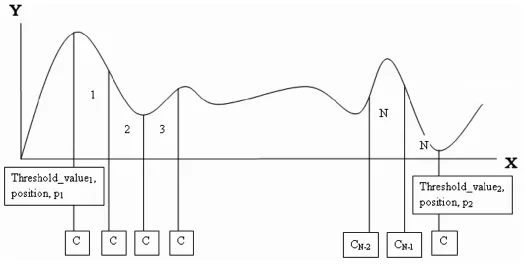
_𝒌𝟐

[image:2.612.54.579.307.571.2]

The calculation of value of C shown in the Figure 1 below:

Fig 1: Total number of intermediate C calculation.

The above histogram is divided into the N no. of section in where C1, C2… CN-1 is denoted as the coordinate of the limit

of each range. The respective value is shown in the Figure 2

below:

[image:3.612.55.579.73.334.2]

Fig 2: Smallest derivational value in-between the position of pair of Cs

The above histogram is shown the median points in between section of the each divided segment. Now, the box region on the

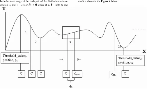
[image:3.612.58.585.407.675.2]

Now, if the no. of division between p1 and p2 is,

𝑵 →

∞. So

the in between range of the each pair of the divided coordinate position is, Cx+1 – C x or

𝑹 → 𝟎

where

𝒙 ∈ 𝑰

+ upto N and

[image:4.612.56.561.86.393.2]

𝑪

_𝒙+𝟏

− 𝑪

_𝒙 are denoted as dx. So, dx → 0. The manipulated result is shown in the Figure 4 below:

Fig 4: variation of mean calculation between every pair of C

Now, the enlarge section of the square box shown in the Figure 5 below:

[image:4.612.53.591.446.646.2]

2.3

Comparison between Integral and Hill

Climbing Constrains

The AB curve portion of the full histogram shown in the before figure has a tangent straight line through the point Z creating an angle θo with respect to X axis.

So, the equation of the straight line is, y = mx + c where

m = tan θ… (1)

And we know tan θ =dy_dx… (2)

Then, comparing (1) and (2) we get: -

m =dy_dx .

Now, putting the value in the equation we get: -

y = dy_dx x + c;

or, y dx = x dy + c dx;

or, x dy = y − c dx.

or, _y−cdy =dx_x;

or, ∫_y−cdy = ∫dx_x ;

The range of the y axis is v1 to v2 and the range of the x axis is

p1 to p2.

∫v2_y−cdy

v1 = ∫

dx x p2

p1

Or, log y − c |v1

v2_{= log x |}

p1

p2

Or, log v2− c − log v1− c = log p2 − log p1

Or, logv_v2−c

1−c= log

p2

p1

Or, v_v2−c

1−c=

p2

p1

So, c = v2∗p_p1−v1∗p2

1−p2

Where, c ≡ C.

So, in the section of dx ∗ dy region the tangent y = mx + c is passing through the point Z of the curvature AB. Now at the

summation of the left areas are the calculation point for the farther proceedings of the iteration and required segmented parts which are denoted by the extra constant value calculated from the straight line equation of the tangent, c. this is the proceeding value of the extra as same as the left portion area of the histogram in each segment. This extra constant value is to be calculated for the margin of the necessary no. of segmentation of the histogram in the total range in between the p1 and p2. So, the calculated region must be between the v1 to v2 for y axis and x1 and x2 for the x axis.

2.4

Proposed Scheme

Threshold_value_selection ( )

{ Threshold_value1=the highest no. of occurrence of the pixel in the image; Threshold_value2=the least no. of occurrence of the pixel in the image;

Where v1=the occurrence value of the pixel at the p1. v2=the occurrence value of the pixel at the p2.

No._of_divided_region, N ≤ (position_highest_frequency_pixel, p1 ~ position_least_frequency_pixel, p2) / constant_value, C.

Where constant value, C = v2 ∗p _p1−v1 ∗p2

1− p2 .

The range of the each divided region is, R = p2~ p_N 1.

For(each_section)

{ Median_position_between(Cx , Cx+1) , Mx= [any_selected_division_position, p1 ± x*R + next_selected_division_position, p1±(x+1)*R] / 2;

Local_minima_at_highest_side, m1=between (median_position, p1 ± x*R); Local maxima_at _least_side, m2=between

(median_position, p1 ± (x+1)*R); } }.

2.5

Approach of Hill Climbing Algorithm

2.5.1

Finding of Local minima at the highest

occurrence value

Between_range (median_position_between(Cx , Cx+1) or Mx ,

Cx)

{ Local_counter1= Local_counter2=0;

Comparison _position1=median_value_position, Mx;

For (i=median_value_position to Cx)

If [f (i-1) = f (Comparison _position1)]

Local_counter1++;

Else

Local_counter2++;

If (Local_counter1=> C OR Local_counter2=> C)

Exit (loop);

}

Threshold_value3=f (comparison_position1);

}

2.5.2

Finding of Local maxima at the least

occurrence value

Between_range (median_position_between(Cx , Cx+1) or Mx ,

Cx+1)

{

Local_counter1= Local_counter2=0;

Comparison _position2=median_value_position, Mx ;

For (j=median_value_position to Cx+1)

{

If [f (j+1) > f (Comparison _position2)]

{

Comparison _position2= Comparison _position2 + 1;

Local_counter1<=0;

Local_counter2<=0;

}

If [f (j+1) = f (Comparison _position2)]

Local_counter1++;

Else

Local_counter2++;

If (Local_counter1=> C OR Local_counter2=> C)

Exit (loop);

}

Threshold_value4=f (comparison_position2);

}

C=constant value defined before.

Where, f(x) = value of the no. of occurrence of the pixel at the „x‟ color level position.

And, constant_value= mean value between threshold_point1 and the median, p2−p₄ 1 .

3.

EXPERIMENTAL RESULT

Typically, it leads to a non-liner optimization problem, the Hill Climbing Algorithm the initial value of calculation used from the median value between the least and highest no. pixel frequency at their cardinality. The Hill Climbing Algorithm is applied to image histogram and the operation of the local minima and maxima concept to find out the median of the threshold value. The proposed algorithm is employed on a remote sensing image of fire in a coal seam at the District of Jhariya, [9] Jharkhand, India. This Hill Climbing Based Histogram Segmentation technique helps to find out the respective area of fire spreading. The fire affected region is manipulated to calculate the fire intensity. The temperature increasing rate can be also recognized in this process. The original image is shown in the Figure 6 below:

[image:6.612.134.477.462.666.2]

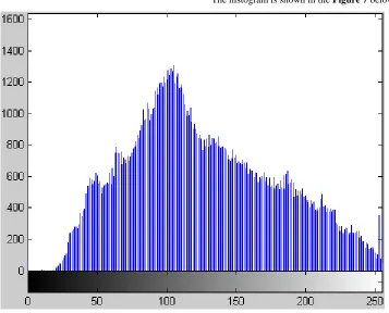
The following histogram shows the red color orientation only.

[image:7.612.130.487.94.382.2]

The histogram is shown in the Figure 7 below:

Fig 7: Red color level histogram

The following histogram shows the Green color orientation only.

[image:8.612.130.486.93.381.2]

Fig 7: Green color level histogram

The following histogram shows the Blue color orientation only. The histogram is shown in the Figure 8 below:

Fig 7: Blue color level histogram

The coal fire image, taken by remote sensing, is segmented by the proposed hill climbing algorithm based multilevel histogram thresholding respectively as blue, green and red.

The blue color based segmentation shows the heat affected area due to coal seam fire. The respective area shown in the Figure 7

[image:8.612.130.485.456.683.2]

below:

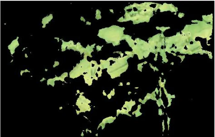
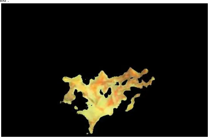
The green color based segmentation represents the probable fire spreading region at the mine area.

[image:9.612.129.487.115.343.2]

The respective area shown in the Figure 8 below:

Fig 8: Possible Fire Spreading Area

The red color based segmentation shows direct fire area at the coal seam of Jharkhand .

[image:9.612.128.486.403.640.2]

An attempt to find out estimated parameters of the distribution will fit the best in given histogram data by using least-square method.

4.

CONCLUSION

The Gaussian Density Distribution function or the Gaussian Fitting Curve method is very effective in the thresholding case, but its computational time becomes deviated in case of multilevel thresholding and it does not work with the individual values of the histogram. To make the evolutionary computation method in the field of independent image segmentation with more perspective, we have proposed a more visible thresholding point selecting scheme called the “Multilevel Thresholding with Hill Climbing Algorithm” that solves the multilevel segmentation process better than Gaussian curve fitting and Gaussian density distribution function in term of computational time complexity. The application of the proposed scheme is implicated on the simulator, MATLAB. To sum up, the Hill Climbing Algorithm with the local minima-maxima concept is a promising and effective tool for image segmentation by multilevel histogram thresholding due to its computation efficiency, and this method proves the effectiveness with respect to the quality performance than previous schemes.

5.

ACKNOWLEDGMENTS

Our thanks is oriented to Krishna Kant Agarwal, Vimal Upadhay and Akhilesh Srivastav who have contributed towards development of the template.

6.

REFERENCES

[1] Glasbey, Yin Zuink, C.A., “An Analysis of Histogram Based Thresholding Algorithm”, 2003.

[2] Fan.S.K, Tsai Yen, S.K.Gonsal, “A New Criterion for Automatic Multilevel Thresholding”, 2008.

[3] Zaraha E, F.J.Chang and G.Bilbro, “Optimal Multi-Thresholding Using Hybrid Optimization Approach”, 2005.

[4] Renders J.M, S.P.Flasse, “Hybrid Method for Genetic Algorithm for Global Optimization”, 2006.

[5] Alexandre Temporel, Tim Kovacs; “A heuristic hill climbing algorithm for Mastermind”, http://www.cs.bris.ac.uk/Publications/Papers/2000067.pdf

[6] Kishor Bhoyar, Omprakash Kakde; “Color Image Segmentation Based On JND Color Histogram”; International Journal of Image Processing (IJIP) Volume(3), Issue(6).

[7] St´ephanie Jehan-Besson, Michel Barlaud, Gilles Aubert, Olivier Faugeras; “Shape Gradients for Histogram Segmentation using Active Contours”; Proceedings of the Ninth IEEE International Conference on Computer Vision (ICCV 2003), Volume – 2.

[8] Dr. Sonali Agarwal, and Prof. G.N. Pandey, “Studies on E Governance in India using Data Mining Perspective”, Journal of Computing, Volume 2, Issue 10, October 2010

[9] Source of Application image –