Three decades of industrialization

(1)

Munich Personal RePEc Archive

Three decades of industrialization

Syrquin, Moshe and Chenery, Hollis

May 1989

Online at

https://mpra.ub.uni-muenchen.de/32771/

(2)

T H E W O R L D B A N K E C O N O M I C R E V I E W , V O L . 3 , N O . 2 : 1 4 5 - 1

Three Decades of Industrialization

Moshe Syrquin and Hollis Chenery

Economists have long searched for patterns that relate successful development to structure and policy. This article reviews the experience of growth and industrialization in the postwar period in more than 100 economies, drawing on time-series data over a three-decade period. Economies are classified according to their population size, the share of primary or manufactured goods in their exports, and the weight of exports in

gross domestic product (GDP). We examine the composition of demand, trade, output,

manufacturing type, and factor use overall and between sectors as they relate to income growth. Higher income growth and more marked transformation are found among the groups with large populations, a predominance of manufactures in exports, and a larger role of exports. We also find that the patterns suggested by cross-country analysis are robust when tested using the time series data now available. Although development experiences may vary over time and across countries, there is sufficient uniformity within them for the main features of structural transformation to emerge as clear and consistent patterns of modern economic growth.

Since its origins in the 1950s, the study of development economics has been concerned with similarities in the way countries grow. Uniform features of the development process, commonly known as "stylized facts of development," have been identified, but significant questions about the common processes remain and are addressed here. We draw on time-series data from three decades of observation to examine whether the patterns emerging from cross-country comparisons of structure and level of development actually reflect transforma-tions that occur over time. This work also brings to light some of the causes of the typical shifts in the composition of production and employment as incomes rise. And finally, we begin to separate out the differential patterns linking economic growth to initial conditions and to development policies.

Early studies on these patterns were conducted by Clark (1940), Kuznets (1957, 1966), Houthakker (1957), Chenery (1960), Temin (1967), and Chen-ery and Taylor (1968). Kuznets identified the transformation of the structure

Hollis Chenery is a professor of economics at Harvard University and a fellow at the Harvard Institute for International Development. Moshe Syrquin is a professor of economics at Bar Dan University, Israel. This article is based on results from research sponsored by the World Bank. Arabinda Kundu and Shujiro Urata were pan of the research team. The authors thank three anonymous referees for useful comments and Yosi Deutsch and Delfin Go for help and advice on the econometric pan.

145

at The University of Miami Libraries on August 12, 2011

wber.oxfordjournals.org

(3)

146 THE WORLD BANK ECONOMIC REVIEW, VOL. 3 , NO. 2

of an economy as the main outcome of "modern economic growth." The comparative approach in the research program that Kuznets initiated was pred-icated on "the existence of common, transnational factors, and a mechanism of interaction among nations that will produce some systematic order in the way modern growth can be expected to spread around the world" (1959, p. 170). The principal transnational factors identifed by Kuznets are systems of produc-tion using technologies derived from the modern sciences, a "community of wants and aspirations," and the emergence of the nation-state in global eco-nomic relations. The way these factors affect the pattern of growth is condi-tioned by such features as a country's size, location, natural resources, and historical heritage.

We made an earlier initial attempt to quantify some of the patterns of "mod-ern economic growth" and the differential effects of initial conditions and development policies on the basis of the 1950-1970 period of rapid growth and relative stability in the world economy (Chenery and Syrquin 1975). We analyzed processes that are commonly used to define structural transformation: accumulation of physical and human capital; shifts in the composition of de-mand, trade, output, and factor use; and such socioeconomic trends as urban-ization, demographic transition and changes in income distribution.

A similar approach was used in the UNIDO studies of industrial change (1979, 1983), McCarthy, Taylor, and Talari's work on trade patterns (1987) and the studies of nineteenth-century patterns of development by Adelman and Morris (1984) and Crafts (1984). Individual country studies of growth and transfor-mation that adopt a comparative approach can be found in Ofer (1987) on the U.S.S.R.; World Bank (1985) on China; and Syrquin (1986, 1987) on Israel and Colombia.

This article draws on much of the earlier work and uses the same analytical framework as our 1975 study. The current work looks only at processes of resource allocation. In the 1975 study two commodity-producing sectors were distinguished: primary and industry. The primary sector is divided here into agriculture and mining, and industry into manufacturing and construction. The relation of the composition of the manufacturing sector to the level of devel-opment is also analyzed, for a smaller sample, extending the results of previous studies (Chenery 1960; Chenery and Taylor 1968; Maizels 1963; and Prakash and Robinson 1979). In this study we extend our data base to 1983. We thus increase the coverage of our time series by more than 50 percent and include the more recent period of slower growth and greater instability. This makes it possible to test the robustness of our principal findings and to obtain more valid comparisons of cross-section and time-series estimates, which is a central issue in this type of analysis.

Patterns of development reflect the association of changes in structure and the level of development. In a cross-country framework, markets and prices are seldom studied directly. Therefore the links to policy are examined using indi-rect methods. Similarly, although the relations uncovered reflect some influence

(4)

Syrquin and Chenery 147

of economic structure on growth, they do not quantify that impact. To do so, it would be necessary to introduce behavior more explicitly and to rely on more country-specific experience.

Patterns of development, based on intercountry comparisons, are average relations. The same overall pattern of transformation can accommodate signif-icant differences in the timing and sequencing of particular aspects of change. Uniformities at a broad level of aggregation can hide wide variation in the behavior of individual components.

Finally, because we examine only the processes of growth, our findings are of little help in analyzing the causes of stagnation in countries with very low income. The average patterns of transformation, however, may serve as indi-cators of feasible paths to growth.

We account for some of these limitations in our analysis here and in other related work (Syrquin 1988). But others are inherent in the analysis and must be recognized as qualifications to it. We will address these limits as they arise in the following discussion.

We begin by outlining the data and procedures used, before reviewing the general patterns of structural transformation in section II. Several hypotheses are examined in section III that link differences in economic growth to differ-ences in initial structure or government policy. Short-term patterns within countries are analyzed in section IV.

I. ECONOMETRIC PROCEDURES AND DATA

In the analysis, we initially estimate the relation of a series of variables reflecting economic structure with the countries' income and population. The available data set covers the period 1950-83 for a maximum of 108 countries (see appendix table A-l at the end of the article). Because the centrally planned economies pursued a unique strategy of urbanization and industrialization that significantly altered their patterns of development in comparison with other economies (see, for example, Ofer 1980) they are excluded from our analysis. We also omit all countries with a population in 1965 of less than 1 million.

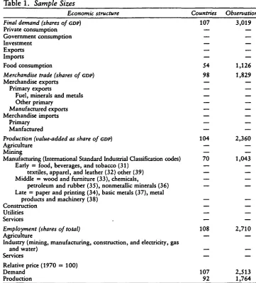
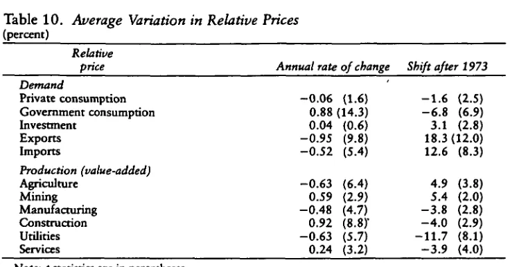
The variables selected reflect intersectoral demand, trade, production, factor use, and relative prices (table 1). They are expressed as shares of GDP, or, in the case of sectoral employment, as shares of the total labor force. Our findings concerning changes in relative, prices are examined in section IV.

To facilitate comparison with previous studies we generally used the same methods as in our earlier work (Chenery and Syrquin 1975). Our basic cross-country regression, estimated for all variables,1 is:

(1) x = a + /S.ln y + j32(ln y)2 + 7,ln N + 72(ln N)2 + E5,T,.

1. We also estimated a variant of equation 1 which included foreign capital inflow, measured by the deficit in the current account as a share of GDP (reported in Chenery and Syrquin 1975; Syrquin and Chenery 1989).

(5)

[image:5.624.188.549.86.485.2]

148 THE WORLD BANK ECONOMIC REVIEW, VOL. 3 , NO. 2.

Table 1. Sample Sizes

Economic structure Countries Observations Final demand (shares of CDP) 107 3,019 Private consumption — — Government consumption — — Investment — — Exports — — Imports — — Food consumption 54 1,126

Merchandise trade (shares of CDP) 98 1,829 Merchandise exports — — Primary exports — — Fuel, minerals and metals — — Other primary — — Manufactured exports — — Merchandise imports — — Primary — — Manfactured — —

Production (value-added as share of CDP) 104 2,360 Agriculture — — Mining — — Manufacturing (International Standard Industrial Classification codes) 70 1,043 Early = food, beverages, and tobacco (31) — — textiles, apparel, and leather (32) other (39) — — Middle = wood and furniture (33), chemicals, — — petroleum and rubber (35), nonmetallic minerals (36) — — Late = paper and printing (34), basic metals (37), metal

products and machinery (38) — — Construction — — Utilities — — Services . — —

Employment (shares of total) 108 2,710 Agriculture — — Industry (mining, manufacturing, construction, and electricity, gas

and water) — — Services — — Relative price (1970 = 100)

Demand 107 2,513 Production 92 1,764

where x = dependent variable (as shown in table 1), y = per capita gross national product (GNP) in 1980 dollars, N = population in millions, and T, = dummy variables for four time periods where Tj = 1 if f > 1960, T2 = 1 if

t z> 1967, T3 = 1 if t 2= 1973, and T4 = 1 if t S; 1979.

The time variables are defined in an incremental way. For example, the coefficient of T2 measures any shift after 1967, over and above the post-1960 shift reflected in the coefficient of Ts. The oil shocks in 1973 and 1979 and the

accompanying changes in the international economy are likely to have created structural changes which are represented by the dummy variables T3 and T4.

We use the semilog formulation because many of the processes we examine seem to follow a logistic or S-type function. In addition, the fitted equations

(6)

and predicted values derived for the components of an aggregate add up iden-tically to the fitted equation and predicted value for the aggregate (provided all estimates refer to exactly the same sample).

Equation 1 was run for pooled samples combining the individual time series for all countries or for groups of countries according to the typologies described below. In general, most of the variance to be explained in these regressions is due to variation among countries, but to a lesser extent than in previous studies. This reduction in the between-country variation is the result of our longer time series and the substantial growth and transformation exhibited in the group of newly industrializing countries since the early 1950s.

The individual time series are also analyzed directly in two ways. Average time-series relations are estimated by allowing each country to have its own intercept:

(2) x = a; + j3,ln y + /32(ln y)2 + E6.T,

where a, = intercept for country /'.

This eliminates all the variation between countries and pools the withcountry variation. The estimated parameters are weighted averages of the in-dividual time-series estimates, with weights related to the variance of the ex-planatory variables. In time series analysis any uniform change is indistinguish-able from a time trend. Population growth would appear only as a trend, and thus it is omitted from the equation.

Individual time-series relations within countries are also estimated in all cases for which a minimal number of annual observations were available. In these regressions only the log of income, In y, appears as an explanatory variable.

The quality of the data is not uniform across countries or over time. All the data come from the World Bank's data tapes and often incorporate adjustments made to remove discrepancies and inconsistencies evident in the original series. Although the series used are probably the best comparable data available for a large number of countries, undoubtedly errors of measurement still remain.

When such measurement errors are random with no systematic component, least-squares estimates are inconsistent and biased toward zero. This does not, however, apply to predictions based on the variables as measured, which re-main unbiased. This problem is compounded when squared terms are used, as occurs with income, y, and population, N, in this study. In such cases the coefficient of the nonlinear term is biased as the square of the bias factor of the linear term. The principal effect of such errors in our study is the underesti-mation of income effects, so that the magnitude of the structural transforma-tion and the strength of nonlinear effects during the process are larger than our estimates suggest.

Systematic nonrandom errors of measurement create effects similar to those arising from model misspecification due to omitted variables. An important instance of such a systematic association in this study is the effect of using exchange rates for converting local currencies to U.S. dollars instead of using

(7)

ISO THE WORLD BANK ECONOMIC REVIEW, VOL. 3 , NO. 2

purchasing-power parities (PPPS) (see Chenery and Syrquin 1986 for a discus-sion of the effects). Attempts have been made to estimate real incomes (con-verted at PPPS rather than at exchange rates) for samples of countries (see, for

example, Kravis 1984). The exchange-rate deviation indexes estimated tend to be higher for poorer countries, so that use of exchange rates rather than PPPS

in comparing GDP tends to undervalue GDP for the low-income countries. The result of relevance for our study is that differences across countries in incomes converted at exchange rates tend to exaggerate the real differences in income. The transformation in the structure of an economy, therefore, takes place over a narrower range of real income than is implied by our estimates.

If the systematic effect causing the error in measurement is expected to continue, then it can be argued that the uncorrected estimates are the more relevant, even though they combine both (real) quantity effects and price ef-fects.

The use of exchange rates may affect differently the various components of GDP. Reports of the International Comparisons Project (ICP) give information on the price structures of the countries studied (for an overview of the project, see Kravis, Heston, and Summers 1982). They show that the relative price of government consumption generally rises with income, whereas the relative price of investment declines. While the ICP does not examine sectoral production, we assume also that the relative price of services tends to increase with income.

The influences of the expected biases strengthen some of our results but qualify or even nullify others. For instance, we find that investment increases with income. The result is strengthened when one accounts for the undervalu-ation of investment at higher income levels created by use of exchange rate rather than PPP conversions. Conversely, the expected bias in valuation of services would undermine our finding that the share of services increases with income. The case of services is further discussed below.

Finally, if the systematic errors of measurement associated with income vary primarily between countries and are relatively invariant within a country over time, then in the average time-series formulation (equation 2) the omitted effects thus implied become part of the country-specific intercept, and correct for the specification bias.

These are the main expected effects from possible errors in measurement. A more extended discussion and references are provided in Chenery and Syrquin (1975, technical appendix).

II. DIMENSIONS OF THE STRUCTURAL TRANSFORMATION, 1950-83

Average growth in total and per capita income during the three decades was significantly higher than in any comparable period in recent history (table 2). Average annual income per capita grew at 2.4 percent. At this rate income per capita would have doubled after thirty years. Of course, the rate was not uniform among countries or groups. Seven of the twenty-nine economies in the

(8)

[image:8.623.74.436.106.199.2]

Table 2. Average Annual Rates of Growth: 1950-83

(percent)

Group

All

Low-income

Lower-middle-income Upper-middle-income Industrial

Number

of

Countries

108 29 29 29 19

Per capita Income

2.4 0.8 1.9 3.6 3.2

GNP

4.6 3.0 4.7 6.0 3.7

Multiple of initial income

per capita after thirty years

2.04 1.27 1.76 2.89 2.57

Note: Growth rates are computed by least-squares regressions for all observations available within a country. Sixty countries had thirty or more annual observations, forty-one countries had between twenty-four and twenty-nine observations, and seven had fewer than twenty-four observations (see appendix table A-l). Libya and Saudi Arabia are included only in the total.

Source: Calculations based on data from the World Bank.

low-income group had negative rates of growth. In the twenty-two with posi-tive growth, the average rate equalled 1.4 percent. Developing countries expe-rienced a clear acceleration of growth as income rose, reaching an average rate of 3.6 in the upper-middle-income group. At this rate the initial income level would increase by a factor of about 3 in thirty years. Several countries multi-plied their starting income level by a factor of 4, or even 5.

This rapid rate of growth means that several countries traversed a large segment of the total range of per capita incomes seen across all countries. Accompanying this growth of income was a transformation of the structure of the economy. In our earlier work, we observed that about 75-80 percent of this transformation took place within the income interval of $100-51,000 in 1964 U.S. dollars (Chenery and Syrquin 1975, p. 19). In this study we define the transition range in 1980 U.S. dollars as the interval from $300 to $4,000 per capita GNP. These revised figures account for inflation since 1964 and reflea the tendency for real exchange rates in developing countries to depreciate relative to the average for industrial economies—and the lower the income level, the greater the depreciation (Wood 1987).

Table 3 shows the predicted values for the shares of the various components of economic structure at different levels of per capita income. These figures are derived by estimating equation 1 for the 1950-83 period for a hypothetical country of average size (N = 20). In calculating the predicted values for the five levels of per capita income we incorporate uniform shifts up to the post 1973 period, but not any shifts after 1979. That is, we set Tt = T2 = T3 = 1

and T4 = 0. (The estimated regressions appear in Syrquin and Chenery 1989.)

Because logistic functions are characterized by upper and lower asymptotes, at the two income extremes ($300 > y > $4,000 in 1970) instead of presenting the predicted values, we calculated the actual average shares for the intermedi-ate period, 1960-72, which was more stable than the lintermedi-ater period, and for which we had higher quality data. The difference between these two extremes,

(9)

[image:9.800.133.704.345.560.2]

Table 3. Shares of Economic Structure Associated with Levels of Per Capita Income

(percent)

^ Component

{3 of economic structure Final demand Private consumption Government consumption Investment Exports Imports Food consumption Trade Merchandise exports Primary Fuels Other Manufacturing Merchandise imports Primary Manufacturing Actual average 000" 79 12 14 16 21 39 14 13 03 10 01 16 05 11

Income per capita (1980 U.S.

300 73.3 13.6 18.4 19.3 24.6 38.7 15.2 13.9 04.8 09.1 01.3 18.2 06.4 11.8 500 70.2 13.5 20.8 20.7 25.2 34.5 16.9 14.9 06.3 08.6 02.0 19.3 06.7 12.6

Predicted1' 1,000 66.4 13.7 23.3 22.6 26.0 29.1 18.8 15.2 07.3 07.9 03.7 20.6 07.1 13.5 2,000 63.1 14.4 25.0 24.5 27.0 23.9 20.3 14.1 07.2 06.9 06.1 21.7 07.5 14.2 dollars) 4,000 60.3 15.4 25.9 26.4 28.0 18.9 21.2 11.8 06.1 05.7 09.4 22.7 08.0 14.7 Actual average > 4,000° 60 14 26 23 23 15 18 07 02 05 11 19 07 12 Total change

- 1 9 02 12 07 02 - 2 4 04 - 0 6 - 0 1 - 0 5 10 03 02 01 Midpoint of change 600 — 400 400 — 1,200 400 — — 1,250 2,000 — — —

(10)

Production (value-added)

Agriculture Mining Manufacturing Construction Utilities Services

Manufacturing

Early Middle Late

Labor force

Agriculture Industry Services

48 01 10 04 06 31 07 02 03 81 07 12

39.4 05.0

12.1 04.4 06.7 32.4

06.8 03.3 01.8

74.9 09.2 15.9

31.7

06.6

14.8 04.9 07.4 34.6

07.6 04.3 03.2

65.1 13.2 21.7

22.8 07.7 18.1 05.5 08.1 37.8

08.3 05.3 05.3

51.7 19.2 29.1

15.4

07.5

21.0 06.1 08.8 41.2 08.3 06.0 07.6 38.1 25.6 36.3

09.7 06.1 23.6 06.7 09.3 44.7 07.8 06.5 10.2 24.2 32.6 43.2

07 01 28 07 10 47 07 06 13 13 40 47

- 4 1 0 18 03 04 16 0 04 10 - 6 8

33 35

700 — 1,200 1,000 900 1,300 — 500 2,500 1,300 1,600 1,000 —Not applicable: change is not monotonic or significant.

Note: Expressed as shares of GDP, except for labor force variables, which are expressed as shares of total labor force. a. Based on 1960-72 period for countries with per capita income less than $300 in 1970; mean approximately $180. b. Assumes average population (20 million).

c. Based on 1960-72 period for countries with per capita income greater than $4,000 in 1970; mean $7,300. Countries with income only slightly over $4,000 in 1970 are excluded: these are Israel ($4,035), Ireland ($4,135) and Spain ($4,310).

Source: Calculations based on data from the World Bank.

(11)

1S4 THE WORLD BANK ECONOMIC REVIEW, VOL. 3 , NO. 2

which is a measure of the magnitude of change as income rises, is also shown. Finally, we indicate the differences in the timing of the change in these compo-nents. The last column shows the level of income at which half of the total structural change has taken place, for variables where change is significant and monotonic.

The evidence presented in table 3 suggests that the uniformity of the struc-tural transformation revealed in our earlier work is quite robust. When we compare the goodness of fit of the former estimates for 1950-70 to the present ones through 1983, the standard errors of the estimates for the two studies are remarkably similar, and when different, they favor the new study (Syrquin and Chenery 1989).

The transformation in final demand is one of the most uniform features of the process of development. On average, the share of private consumption in GDP declines with the level of income, as the share of investment rises and the trade deficit declines. Food consumption drops by about 20 percentage points, while nonfood consumption (not shown separately) goes up. The shift from consumption to investment takes place at a lower income level; the decline in food consumption is spread over a wider income range.

Only a small part of the variation in aggregate trade can be related to income. In the composition of exports we do find a fairly steady increase in manufac-tures throughout and a decline in the share of primary products in the later periods. No such change takes place in imports, for which there is an increase in both components. Only in large countries do we find a decline in manufac-tured imports, which is clearly related to early import substitution.

Changes in final demand and trade reinforce each other. They combine with complementary changes in intermediate uses and productivity growth to pro-duce a more pronounced shift in the structures of production and labor use.

The share of value added in agriculture declines sharply over the transition, whereas manufacturing, construction, and utilities double their share and the services sector share rises by about 50 percent. It has been argued that the rise in services is wholly a product of increasing services prices (Kravis, Heston, and Summers 1983). Although there is a significant price effect in the rising share of services, we will show in section IV that it does not account for all of the increase.

For the earlier period, the rising industrial output share surpassed the declin-ing primary share at an income level of approximately $300 (1964 U.S. dol-lars), when both industry and the primary sectors accounted for about 26 percent of total value added. The same transition point was reached in the present study at an income of $1,500 (1980 U.S. dollars), when the two sectors equal about 25.5 percent of output. The rise in manufacturing and industry production shown here is smaller than that found for earlier periods, probably reflecting the deindustrialization of the developed countries.

The decline in the share of agriculture in employment is more pronounced than in production, but since it starts from a much higher level its percentage

(12)

decline is smaller than for agricultural production. Thus the relative productiv-ity of labor in agriculture (share in value added divided by share in employ-ment) drops through income levels of around $3,000 before the gap in average productivity begins to narrow.

The sectoral correspondence of the structures of demand, trade, and produc-tion in table 3 is only approximate. Strict comparability would require match-ing the classification schemes (International Standard Industrial Classification, and Standard International Trade Classification), and an interindustry frame-work to allocate expenditure categories to industries and to account for inter-mediate goods.

Over the course of the transition there is a significant shift in value added from primary production to manufacturing and nontradables. For each sector we analyzed the sources of this shift arising from changes in the composition of demand for intermediate and final goods and from changes in net trade (Syrquin and Chenery 1989). The average patterns thus derived show a very close correspondence with those shown in the directly estimated shift (table 3). Changes in domestic demand (Engel effects) seem to account directly for less than half of the change in structure, and changes in net trade for about 10 percent on the average.

Changes in the use of intermediate inputs as income rises push down the share of primary-sector value added in two ways (information on intermediate production comes from a comparative study of interindustry relations by Deutsch and Syrquin, forthcoming). First, as income rises, producers in all sectors substitute manufactured inputs for natural intermediates because of changes in prices and production technology, accounting for around 15 percent of the decline in the primary sector share. Second, producers in the primary sector increase their use of inputs relative to output, reducing the ratio of value added to gross output. About one-fourth of the decline in the share of primary sector output results from this increase in the use of inputs in the primary sector. In an input-output model, the variation in intermediate use can be further attributed to changes in final demand, trade, and input-output coeffi-cients (see, for example, Chenery, Shishido, and Watanabe 1962, for Japan, or Chenery and Syrquin 1980 and 1986a, for a cross-country analysis).

Manufacturing: Disaggregated Results

During the process of industrialization, the composition of the manufactur-ing sector changes considerably. At a less aggregated level, country-specific features and policy become more prominent in determining the pattern of specialization. Large countries can better exploit economies of scale within their domestic markets and can more easily afford a strategy of import substi-tution. Variation in resource endowments is expected to generate differences in production patterns within manufacturing, particularly in small economies. Nevertheless, various studies have shown that a high degree of uniformity still remains in the pattern of change within the industrial sector.

(13)

There have been various attempts in the literature to group industrial sectors into homogeneous categories differing in their technology, their dynamism, or the demand for their produrts. Hoffmann (1958) stressed the systematic decline in the ratio of consumer to producer goods. At the Economic Commission for Latin America (1964) the labels became more emotive: dynamic and vegetative branches. In this study nine industrial branches were distinguished. The results in table 3 are aggregated into three industry groups "according to the stage at which they make their main contribution to the rise of industry" (Chenery and Taylor 1968, p. 409). Early industries are established at low income levels to satisfy the essential demands of the population (food, textiles, clothing). They are characterized by simple technologies and low income elasticities of demand. Their share in GDP remains static during the transition at an average about 7-8 percent. Within manufacturing their share goes down significantly, although there are some recent exceptions where the output of some branches in this group expanded rapidly for exports.

Middle industries typically double their share in GDP early in the transition, from about 3 percent to 6 percent, but show little further increase. A large proportion of their output is used as intermediate inputs by other sectors (chemicals, nonmetallic minerals). This source of demand expands at lower income levels when the matrix of interindustry relations becomes more dense. Income elasticities for the finished produrts from the group of middle industries are generally above unity.

The group of late industries accounts for virtually all of the increase in the manufacturing share in the latter stages of the transformation. This group includes investment goods (machinery), some intermediates (paper), and dura-ble consumer goods with high income elasticities of demand (metal products). At low income levels this group typically accounts for less than 3 percent of GDP, whereas by the end of the transition it commonly reaches or exceeds 10 percent of GDP.

Shifts over Time

Some long-run processes of change proceed over time independently of vari-ations in income. For example, changes in the level of technology, the interna-tional environment, or the strategies of development may lead to shifts in the dependent variables. To the extent that those long-run processes of change can be assumed to be universal and to affect all countries alike, their effect would be captured by the time dummy variables in equation 1. In a more general model the time-shift variables would be replaced by the processes for which they stand as proxies.

Some of the omitted variables vary primarily among countries and are rela-tively invariant within a country over time. If these variables are correlated with income across countries, the cross-country patterns will differ from time-series estimates and this difference may end up as part of the time trend in the intercountry estimates.

(14)

Finally, we have the case of random or unanticipated shocks, such as the quadrupling of the price of oil in 1973. If the impact of the shocks is uniform for all countries, it will appear in the time-shift variable. If it is random, it may impair the accuracy of the estimates. When the impact of the shock is different for different groups of countries, an additive time-shift variable will fail to represent the differential effect. If there is reason to believe that the effect of the change (in oil prices for example) varies systematically with income or some other characteristics, we could introduce interaction terms or split the sample to estimate separate regressions for the time periods before and after the change, and compare predicted values at various income levels.

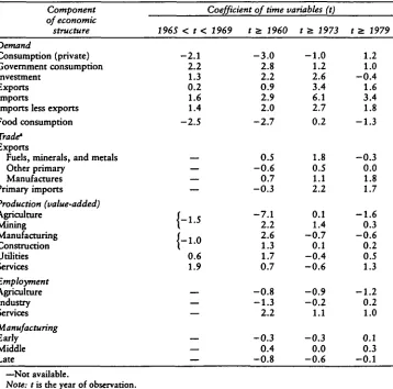
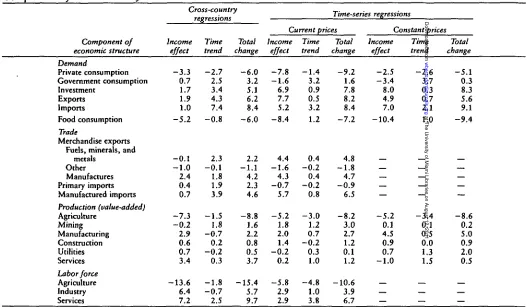
[image:14.619.81.439.275.629.2]

The uniform time shifts up to the late 1970s shown in table 4 reinforce the income-related decline in food consumption and rise in investment, government

Table 4. Uniform Time Trends in Economic Structure, 1950-83

(percent) Component of economic structure Demand Consumption (private) Government consumption Investment Exports Imports

Imports less exports Food consumption

Trade"

Exports

Fuels, minerals, and metals Other primary Manufactures Primary imports Production (value-added) Agriculture Mining Manufacturing Construction Utilities Services Employment Agriculture Industry Services Manufacturing Early Middle Late

1965 < t<

-2.1 2.2 1.3 0.2 1.6 1.4 -2.5 — — — f

j - 1 . 5

( . \ 0.6 1.9 — — — — — —

Coefficient of time variables (t)

1969 t a 1960

-3.0 2.8 2.2 0.9 2.9 2.0 -2.7 0.5 -0.6 0.7 -0.3 -7.1 2.2 2.6 1.3 1.7 0.7 -0.8 -1.3 2.2 -0.3 0.4 -0.8

t s» 3973

-1.0 1.2 2.6 3.4 6.1 2.7 0.2 1.8 0.5 1.1 2.2 0.1 1.4 -0.7 0.1 -0.4 -0.6 -0.9 -0.2 1.1 -0.3 0.0 -0.6

t s 1979

1.2 1.0 -0.4 1.6 3.4 1.8 -1.3 -0.3 0.0 1.8 1.7 -1.6 0.3 -0.6 0.2 0.5 1.3 -1.2 0.2 1.0 0.1 0.3 -0.1 —Not available.

Note: t is the year of observation. a. Data start in 1962.

Sources: Chenery and Syrquin (1975); calculations based on data from the World Bank.

(15)

158 THE WORLD BANK ECONOMIC REVIEW, VOL. 3 , NO. Z

consumption, trade shares and trade deficits. The large shift from agricultural production to all other sectors in the pre-19.73 period can be explained by the nature of technological progress and the substitution of fabricated products for natural materials. The exogenous shift after 1979 from tradables to nontrada-bles combines the effects of the depression and worsening terms of trade in oil-importing countries, with the changes in structure in oil-exporting economies known as "Dutch disease." Dutch disease results when a sudden drastic increase in foreign exchange earnings leads to currency appreciation and to an increase in the relative prices of nontradables. As a result exports become less competi-tive and, in general, output and employment in the tradable sectors fall.

To evaluate the uniformity of the time trends, separate regressions were run for the pre-1973 and post-1973 periods and predicted values compared at three income levels: $300, $1,000, and $4,000 (Syrquin and Chenery 1989). In general the predicted values for the two periods are not very different, so that the hypothesis of homogeneity cannot be rejected. The most significant non-uniform shifts are related to trade. The increase in manufactured and total exports after 1973 (holding income and size constant) is positively correlated with income, whereas the import surplus increases most at low income levels. The shares of manufactured output and industrial employment are almost the same before and after 1973 at low and middle incomes but fall significantly in the richer countries. The counterpart is a positive time shift in services employ-ment in advanced countries.

III. TYPOLOGY OF DEVELOPMENT PATTERNS

We review here the average patterns of economic transformation related to the initial conditions and policy objectives of each country studied. We consider some of the factors that lead to diversity in patterns of resource allocation, and we classify countries into more homogeneous groups by population size, share of manufactures in exports, and share of exports in GDP. We exploit the large samples to estimate separate regressions for each group, and we then define a typology of development strategies.

Country Classification

Countries are classified first as large or small based on their population in 1965. We then divide countries into two groups according to the predominance of primary or manufactured goods in their exports. This commodity composi-tion is reflected in a trade orientacomposi-tion index (TO), which substracts the predicted difference between primary and manufactured exports (as a share of total merchandise exports) from the actual share:

TO = (EP - EM)/EMR - (EP - EM)/EMR

where EP, EM, and EMR are primary exports, manufactured exports, and mer-chandise exports respectively, and the hat over a variable refers to predicted

(16)

Syrquin and Chenery 159

values.2 The TO index was calculated for data from 1965 and 1980 on the basis of separate regressions by country size (small and large) and period (pre- and post-1973). Countries with positive TO values were classified as primary-oriented

and countries with negative TOS as manufacturing-oriented.

We also classify countries according to their observed share of merchandise exports in GDP relative to the predicted share for 1965 and 1980, on the basis of separate regressions by size and period. A high relative export level led to an

outward classification whereas a low level resulted in an economy being classi-fied as inward.

Although the relative export level is much influenced by trade policies, our simple measure of openness is not directly based on policy instruments but on realized levels of trade. Some studies rely directly on the policy variables for identifying trade strategies. A recent example is the analysis of trade orientation in World Development Report 1987. However, such a classification tends to vary significantly over time and, by ignoring initial conditions, implicitly as-sumes an unrealistic degree of flexibility in the structure of the economy. The correspondence between the typology in the World Development Report and the one below nevertheless is quite high. We aim to identify significant differ-ences among broad groups and to provide relevant benchmarks for country analysis. For these purposes reclassifying a few countries among the types has only a marginal effect on the results.

All countries in our sample were classified on the basis of the three factors: size, specialization, and openness (see appendix table A-l). In the great major-ity of cases the classification resulted from adherence to fixed sets of criteria: one for small countries and one for large ones. But, the computed indexes for 1965 and 1980 at times gave conflicting results. Where a clear shift between the two points could be discerned, we gave a larger weight to the position in the terminal year in classifying the country for the whole period. In addition, the indexes of specialization and openness are based on merchandise exports only. In some cases we also considered exports of services and the trade balance as shares of GDP, especially where extreme values of the variables were recorded and where the classification was not a clear-cut one. (For more details on the classification see Syrquin and Chenery 1989.)

Variations in Patterns of Resource Allocation

Many of the variations from the average patterns of growth are a reflection of the interaction of comparative advantage with policy. For example, a great relative abundance of natural resources that are economical to exploit at given prices and technology (especially oil and other minerals), is expected to lead to a high share of primary exports. Although it is difficult to measure the availa-bility of resources, a simple proxy for the proportion of resources to population

2. There are small definitional changes from the 1975 analysis that have little effect on the general conclusions. The TO index is illustrated in greater detail in Chenery and Syrquin (1986b).

(17)

1 6 0 THE WORLD BANK ECONOMIC REVIEW, VOL. 3 , NO. 2

is the density of the population. A high density has been shown to be signifi-cantly associated with lower trade shares and a higher share of manufactured goods in total exports (Perkins and Syrquin 1989).

The level of income affects the composition of exports in two ways. First, a higher income level is associated with greater absorptive capacity, so there is less surplus to be vented. Second, the ratio of capital (physical and human) to labor is positively associated with per capita income. As a country develops it tends to go through "stages of comparative advantage" moving from resource-intensive commodities to labor-resource-intensive and then to more capital- and skill-intensive goods (Balassa 1979, Learner 1984). Although the share of total exports seems to be only weakly associated with the level of income, the commodity composition shows a significant shift from primary to manufac-tured exports.

' Size and specialization. We identify four categories of countries: small pri-mary, small manufacturing, large primary and large manufacturing. Separate regressions were run for each group, and a summary of the most salient con-trasts appears in table 5. The first column shows the expected level of a variable at an income of $1,000 derived from the average patterns in section II. The last four columns give the ratio of predicted levels from group-specific regres-sions to the average figures in the first column.

Large countries export a much smaller share of output than small ones. Among large countries there are significant differences. In the typical large primary-exporting (LP) countries, the relative abundance of natural resources is reflected in its trade composition. Many countries in this group followed an import substitution strategy for a large part of the period after 1950. One result of this policy was a failure to develop manufactured exports, which also shows up in the smaller share of industries classified as "early" and in the relatively low share of industrial employment. By contrast, among the large manufac-tured (LM) goods exporters, the overall share of exports is still low but manu-factured exports are substantially higher than in the average pattern, as is the share of early industry in GDP. The exploitation of economies of scale is reflected in the high shares of investment and of middle and late industries.

In small countries trade is more important, but in the small primary-export-ing (SP) economy, primary exports more than offset the shortfall in manufac-tured exports. In the small manufacmanufac-tured good exporters (SM), however, the high level of manufactured exports is accompanied by a high share of primary and manufactured imports. The high level of manufactured imports reflects input requirements, as well as final imports which are a concomitant of the higher degree of specialization and integration in the international economy of the resource-poor SM country.

For the average economy it was shown in table 3 that the major source of growth in manufacturing during the transition is in the late industries, charac-terized by high capital intensity and economies of scale. When we analyze

(18)

[image:18.626.79.444.105.427.2]

Table 5. Index of Shares of Economic Structure of Country Groups Relative to Average Shares

Component of economic

structure Merchandise trade

Exports

Fuels, minerals, metals Other primary Manufactured Imports Primary Manufactured Demand Exports

Imports less exports Investment Production (value-added) Agriculture Mining Manufacturing Services Employment Agriculture Industry Services Manufacturing Early Middle Late Average share" 7.3 7.9 3.7 7.1 13.5 22.6 3.4 23.3 22.8 7.7 18.1 37.8 51.7 19.2 29.1 8.3 5.3 5.2 Primary 125 147 49 97 113 115 76 91 102 109 85 108 112 83 90 106 66 61

Country size and export specialization Small Manufactured Primary 18 106 389 177 180 141 341 105 105 66 95 104 85 123 111 90 79 85 78 63 35 52 67 63 50 98 113 109 97 96 102 88 104 86 96 96 Large Manufactured 19 29 262 152 74 67 221 120 93 43 116 102 89 132 98 113 123 163

Note: Shares calculated are percent of GDP except for employment variables which are shares of total labor force. Index is share for group divided by average share, times 100. Values over 100 indicate a share for that group and economic component that is greater than that predicted for the average; values below 100 reflect shares less than the average.

a. The average share is the predicted share for countries with per capita income of $1,000, based on regressions for the whole sample.

changes in the four groups, this result still holds, except for the SM group, in which the development of labor-intensive exports of manufacturers leads to an expected rise in the share of early industries of about 5 percentage points in the range $300 to $4,000 (for details, see Syrquin and Chenery 1989).

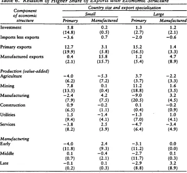
Export share. In the four-way typology analyzed above the degree of open-ness has not been explicitly considered. Further splitting the types would reduce the samples too much for statistical analysis. To assess the average effect of our openness measure (the relative share of merchandise exports in GDP) on the patterns of resource allocation, we add a dummy variable for openness to the regressions within the four types. The variable equals one for countries

(19)

[image:19.621.184.549.87.426.2]

Table 6. Relation of Higher Share of Exports with Economic Structure

Component of economic

structure

Investment

Imports less exports Primary exports Manufactured exports Production (value-added) Agriculture Mining Manufacturing Construction Utilities Services Manufacturing Early Middle Late Primary 5.8 (14.8) -3.6 12.7 (19.9) 0.4 (2.1) -4.0 (6.2) 7.8 (13.5) -2.4 (7.9) 0.9 (6.5) 1.5 (9.4) -3.8 (8.2) -4.0 (11.8) 0.1 (0.7) -0.1 (0.2)

Country size and export specialization Small Manufactured 0.2 (0.5) 0.7 3.1 (5.8) 15.8 (15.7) -5.3 (7.2) 0.1 (0.4) 4.2 (7.5) -0.2 (1.1) -1.4 (4.1) 2.5 (3.9) 2.4 (9.3) -0.4 (2.1) 0.1 (0.3) Primary 1.3 (2.7) -2.0 15.2 (16.5) 1.2 (5.4) 3.7 (3.7) 11.2 (18.8) -9.0 (20.5) 0.1 (0-4) -1.3 (7.0) -4.7 (6.4) -3.1 (11.2) -2.7 (11.7) -2.9 (8.8) Large Manufactured 1.2 (2.1) - 0 . 6

1.4 (3.3)

4.7 (8.9)

- 2 . 2 (3.3)

1.6 (3.5)

3.2 (4.5) - 0 . 2

(0.9) 1.0 (4.1) - 3 . 4

(4.9) 0.0 (0.0) 0.1 (0.3) 3.2 (8.9)

Note: Values are coefficients of dummy variable for group with high share of merchandise exports in GDP; (-statistics are in parentheses.

fied as outward (in appendix table A-l). The coefficient of the dummy variable indicates the added effect of openness after controlling for size and specializa-tion (table 6).

Some of the results follow trivially from the way we have classified countries. Thus trade ratios are strikingly higher in the more open subgroups. Greater merchandise exports are associated with lower trade deficits and higher invest-ment shares, implying higher saving proportions. In the SP group the expected difference in the share of investment is close to 6 percentage points.

The relation with the degree of industrialization differs according to the type of specialization. In primary-oriented countries greater merchandise exports are associated with larger mining shares and lower shares of manufacturing, partic-ularly among large countries. This pattern reflects the combined effect of the import-substitution strategy in inward-oriented countries, and the Dutch dis-ease syndrome in mineral exporters.

(20)

In exporters of manufactures, the more open the economy the larger the share of industry in output. In the small economy (SM) this increase is located in early-light industries while in the large economy (LM) it appears as higher shares of late-heavy industries.

Structures and Strategies

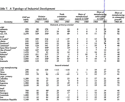
We have classified economies into four general types according to their struc-tural features and trade policies. The typology includes developing countries that are far enough into the transition to identify the strategy being followed and that have the data required for classification. The fifty economies in table 7 include all those identified as semi-industrial on the basis of the contribution of manufacturing to the growth of commodity production (the industry index); per capita GNP; and the share of manufactures in exports and production. It also includes some countries that satisfy only two or even one of the criteria, to enlarge the coverage of the classification (Chenery and Syrquin 1986b). Because the approach used here follows that of our earlier work, and the results of that work appear to be robust, we describe here only the main features of the strategies and structures.

Outward, primary-oriented economies. The countries in this category have very high export shares made up almost completely of primary commodities. The strong primary specialization appears to originate more in resource endow-ment than in a deliberate policy choice.

The continued primary specialization into the advanced phase of the transi-tion can be characterized as a strategy of delayed industrializatransi-tion. The pro-duction and exports of labor-intensive manufactures tend to lag in primary-oriented economies. (For a review of the development experience of such econ-omies, see Lewis 1989.)

All the agricultural exporters are small economies. Large countries that might have been classified in this group in the past have usually pursued a strategy of inward development through import substitution. Among the most successful examples of an outward, primary-oriented strategy is Malaysia. It has main-tained relatively neutral incentives among sectors; the result has been substan-tial growth of manufactured exports while primary exports have stayed at a i high level.

The three large economies are mineral exporters. At low income levels (In-donesia and Nigeria) the abundance of mineral resources dominates the effects of large size which would normally lead to low shares of trade and high shares of manufactures in exports.

The cases of Indonesia and Nigeria illustrate well the importance of struc-tural characteristics for determining a development strategy. In a study of very large countries (Perkins and Syrquin 1989), Indonesia and Nigeria had to be treated separately. Their patterns of development resembled more those of small economies than those typical of large ones. World Development Report

(21)

[image:21.801.194.683.157.559.2]

Table 7. A Typology of Industrial Development Economy Large Indonesia Nigeria Iran, I.R. Small Sri Lankad Liberia Honduras'* Cameroon11 Papua New Guinea*1 C6te d'Ivoired Ecuador Malaysia*1 Algeria Iraq Venezuela Large manufacturing India China Pakistan Large, primary Colombia Turkey Argentina Mexico Small Bolivia Nicaragua Guatemala Peru Dominican Republic GNPper capita, 1980 470 990 2,270 270 520 640 740 820 1,200 1,470 1,650 2,100 3,000 3,800 240 290 310 1,280 1,310 1,980 2,620 760 790 1,080 1,120 1,160 Relative export 1965 80 207 129 309 151 109 124 57 147 77 211 90 155 134 62 70 53 40 46 50 85 80 77 62 56 level 1980 270 171C 210c 216 155 143 141 109c 141' 95 217 118 208' 122 120 82 72 37 32 22C 88° 67 88 84 61 Trade orientation 196S Outward, 7 24 35 - 2 12 21 17 14 32 34 17 24 50 39 index" 1980 primary-oriented 22 49' 89 - 3 7 24 20 29 33C 1' 54 2 31 62' 33 Inward-oriented - 1 1 5

- 5 4 11 25 33 25 26 24 10 28 31

- 1 1 8 - 6 9 23 8 29 14' 43C 17 5 - 1 5

12

Share of manufactured exports in GDP 1962 0 1 1 1 2 0 1 1 0 0 2 1 0 2 2 2 0 0 0 1 1 1 1 0 0 J9S0 1 0 0 5 2 4 1₁ 4 3 1 10 0 0 1 3 5 3 2 1 2 1 3 5 3 3 Share of manufacturing value-added in 1 1960 9 5 11 15 4 12 10 4 7 16 9 8 10 11 14 26 12 17 13 32 19 15 16 13 24 17 SDP 1081 12 6 11 16 8 16 8 9 12 11 21 11 6 15 17 37 17 21 22 25 22 14 26 18 28 16 Share of manufacturing in commodity growth**. 1960-80 30 28 42 38 17 40 40 — 47 46 48 38 26 80 37 72 41 49 55 79 75 46 53 47 67 51

(22)

Paraguay Syria Chile Uruguay Large Egypt, A.R. Thailand Philippines Brazil Spain Small El Salvador Morocco Tunisia Costa Rica Greece Ireland Large Korea, Rep. South Africa Yugoslavia Small, outward Kenya Taiwan Singapore Hong Kong Small, inward Jordan Portugal Israel 1,360 1,510 2,400 3,540 580 710 730 2,000 5,600 740 950 1,370 2,050 4,300 5,100 1,600 2,670 3,050 410 2,270 4,500 5,470 1,140 2,460 4,750 43 54 57 53 105 90 103 120 40 112 70 62 59 22 96 39 135 94 148 314 218 50° 85 41 35C 67C 69 28 138 132 111 58 57 137 57 105 56 3S 125 157 186 75 108 378 220 55 76 82 16 20 46 47 IT 43' 40 - 4 Balanced - 2 5

7 8 30 4 2 1 - 1 6 27 1 22 - 1 1 - 2 7 - 6 - 2 9 - 2 1 - 4 2 - 1 0 - 1 1 - 1 6 - 3 3 Industry-oriented

- 9 6 - 1 8 - 7 4

- 2 0 - 2 6 - 1 1 3 - 2 1C - 8 4 - 6 6

- 1 1 2 - 7 1

-57

- 3 0 - 3 6 - 9 4 - 1 8 - 7 8 - 8 0

1 1 0 0 2 1 1 0 1 2 1 1 2 1 7 1 7 6 2 — 49 1 7 8 1 1 2 4 2 6 6 5 7 11 3 9 8 5 27 23 26 10 3 — 66 6 14 23 17 21 21 21 18 13 20 26 26 14 16 8 14 16 17 14 21 29 9 22 12 22 12 22 23 17 12 22 22 8 20 25 27 24 14 18 14 19 19 23 29 23 25 13 40 30 23 14 30 23 41 36 60 71 48 53 52 82 85 53 59 41 63 71 66 79 63 48 90 96 100 46 95 77 —Not available.

a. Indicates the predominance of primary or manufactured goods in merchandise exports, with positive values reflecting a primary and negative a manufacturing orientation.

b. Termed "industry index" in our earlier works. c. 1975.

d. Agricultural exporters.

(23)

166 THE WORLD BANK ECONOMIC REVIEW, VOL. 3 , NO. 2.

1987 classifies Indonesia as "moderately inward" during 1973-85 and Nigeria as "moderately inward" in the first period and then "strongly inward" in the second. As far as the system of incentives is considered, the classification appears to be accurate, but it ignores the abundance of natural resources that leads to the relatively high export and low manufacturing shares in these countries. Thus, the structures of their economies suggest that Indonesia and Nigeria are best classified as "outward, primary-oriented."

Most mineral (oil) exporters evidenced some signs of Dutch disease in the wake of the sharp increases in the price of energy. The share of mining in output increased at the expense of both manufacturing and agriculture (Ecua-dor, Iraq, Venezuela).

Inward-oriented economies. Among large, inward-oriented countries, two groups can be distinguished. The first comprises three very large countries of Asia with relatively low incomes. The second includes the large countries of Latin America plus Turkey. The Asian group has substantially lower incomes and has a poorer endowment of natural resources reflected in the much higher density of population.

The main difference between the Asian and Latin American economies is in their trade orientation. The large Asian economies here fall into the manufac-turing-oriented category while Latin American countries start with a strong primary orientation. By 1980, however, in most Latin American countries manufactured exports had risen appreciably. This development of manufac-tured exports, hastened by the debt crisis of the 1980s, may not be unrelated to the earlier phase of inward-looking industrialization, during which the econ-omy acquired a basic technological mastery which then facilitated the exporting of manufactures on a significant scale. Teitel and Thoumi (1986) argue that in the large countries of Latin America import substitution provided a preamble to the export stage. Bruton (1989) also calls for a more balanced appraisal of the import-substitution strategy.

Balanced economies. The countries in this group, except Egypt,3 shifted from a primary to a manufacturing specialization in trade, while in most cases maintaining or increasing their normal trade shares. The difference between this group and the inward-orientation group is one of degree because both made extensive use of protection, even during the opening episodes.

Industry-oriented economies. The trade policy of these economies has been mostly outward-oriented, particularly in the Asian economies in the group (Republic of Korea, Taiwan, and the city-states of Hong Kong and Singapore). In most cases the rapid rise in manufactured exports followed an earlier phase

3. In Egypt between 1962 and 1980 the share of fuels, minerals, and metals in merchandise exports rose from 4 percent to 69 percent. In addition, by 1980 remittances and earnings from the canal allowed a deficit in the current account exceeding 15 percent of GDP.

(24)

of import substitution behind high protection. The initial inward-looking poli-cies continued for a relatively short period in Korea and Taiwan; in Israel they were supplemented by export-promotion policies.

Performance

Among the alternative development patterns we categorize, the one that has elicited the most interest has been the relation between performance and the inward-outward distinction. Studies have found a significant positive relation between an outward orientation and strong macroeconomic performance, growth, efficiency in resource allocation or reallocation, higher labor absorp-tion and factor productivity, and adjustment to external shocks (see for exam-ple, Balassa 1989, Krueger 1983, Feder 1983 and 1986, Chenery 1986, and World Bank 1987).

Besides the inward-outward distinction, we considered size and specialization and ended up with eight subgroups. This permits us to make four comparisons of average performance between economies we classify as less and more open with different combinations of initial conditions. Table 8 shows the average growth rate and sample size for the countries in each of the eight subgroups (as listed in appendix table A-l) based on data for 1950-83.

In each case, GDP growth is higher in the outward group, the difference between the outward and inward subgroups varying from a maximum of 1.4 percentage points for small primary exporters down to 0.2 points for large primary exporters. As for the other classifying criteria (size and specialization), the results are less conclusive but still indicate that a manufactured specializa-tion performed better than a primary specializaspecializa-tion and that large countries grew faster than small ones (for the relation of size and performance, see Perkins and Syrquin 1989). However, most of the very fast growers during this period were small or medium-size countries. The smaller countries, being more

Table 8. Annual Growth Rate of GDP by Subgroups, 1950-83

(percent)

Country group All

Primary

Inward Outward

Manufacturing

Inward Outward

Countries (number)

10 5 6 8

Large

Growth rate

5.02 5.00 4.94 5.12 5.04 4.73 5.26

Countries (number)

27 23 17 10

Small

Growth rate

4.54 4.24 3.58 5.01 5.11 4.74 5.73

All

Growth rate 4.67

4.42

5.09

4.28 5.22 Note: Growth rates within countries are ordinary least-squares estimates. The number of annual observations varies from 14 to 34 (see appendix table A-l).