The Adaptability of Decision Tree Method in Mining
Industry Safety Data
Vincent I. Nnebedum
Ph.D
Department of Electrical and Electronics Engineering
Federal University of Technology Owerri NIGERIA.
ABSTRACT
Data Mining nowadays is extensively applied in researches and business fields. The choice of data mining tools is practically dependent on the nature of the data to be mined. Studies have shown that certain tools perform better in certain types of dataset. This paper x-rays a typical real life incident dataset common to oil and gas industries and how decision tree algorithm fits into mining it. The application of Decision Tree mining tool on a real-world safety records perfectly reveals useful information that are subsumed in the volume and nature of the data. The concept of Entropy and Information Gain theory are used in building the decision tree model and an accuracy of 71.4% arrived at, indicating a good performance of decision tree induction on the dataset. Further areas of research on the use of decision tree method in data mining are recommended.
Keywords: Data mining, Classification, Decision Trees,
Prediction, Safety data.1.
INTRODUCTION
Data mining is a process of extracting hidden relationships and patterns in data and delivering results that can either be utilized in an automated decision support system or easily accessed by a human analyst [1]. Several data mining tools have been developed for mining data, but studies have shown that certain tools perform better in certain type of dataset or environment [2]. In fact, no single data mining tool produces same result on all kinds of data set.
Safety data, especially those collected from oil & gas industries, have peculiar characteristics inherited from their sources, utility, behaviour and descriptions. The focus here is on the adaptability of decision tree as a data mining tool on a typical real life incident (safety) data.
Decision tree is an aged method in statistics and machine learning [3]. Literatures on decision tree induction are available in many data mining text books including [4], [5] and [10] referenced. Emphasis in this paper is on the practical application of decision tree classification on a set of safety data. It connotes the use of the derived relationships (or rules) in making real-world predictions. We demonstrated it here by predicting the likelihood of an incident occurring in a particular location of the industry, based on the previous recorded incident occurrences.
2. METHODOLOGY
Data mining uses algorithms or set of rules,and here called models, toextracts the hidden information [6]. Decision Tree (DT) is just one type of data mining’s classification models. Others are discussed in [8], [9] and [10]. DT has the following advantages:
It provides model transparency so that a business user and analyst can understand the basis of the model's
Its algorithm provides speed and scalability. The built algorithm scales linearly with the number of predictor attributes and on the order of nlog(n) with the number of rows, n.
Scoring is very fast. Both build and apply are parallelized. It builds models for binary and multi-class targets, and produces accurate and interpretable models with relatively little user intervention.
Decision tree algorithm is implemented in such a way as to handle data in the typical data table formats, to have reasonable defaults for splitting and termination criteria, to perform automatic pruning, and to perform automatic handling of missing values [8].
The parameters that define the model are the set of attributes that comprise the input vectors, and hence are in the same vocabulary as the domain attributes. With syntactic transformations, they can be put into sets of "IF-THEN" rules that allow for "explanation" of the classifier's reasoning in human terms.
Iterative Dichotomiser 3rd edition, popularly called ID3, is one
of the widely used algorithms of decision tree induction [10]. Other types of DT are detailed in [9]. ID3 constructs decision tree in a top-down recursive divide-and-conquer manner. The ID3 strategy is simplified as follows:
1. The tree starts as a single node representing the training samples.
2. If the samples are all of the same class, then the node becomes a leaf and is labelled with that class.
3. Otherwise, the algorithm uses an entropy based measure known as information gain as a heuristic for selecting the attribute that will best separate the samples into individual classes.
4. The algorithm uses the same process recursively to form a tree for the samples at each partition. Once an attribute has occurred at a node, it need not be considered in any of the node’s descendants.
5. The recursive partitioning stops only when any one of the following stopping conditions is true:
All samples for a given node belong to the same class.
There are no remaining attributes on which the samples may be further partitioned. Hence, majority voting is employed. This involves converting the given node into a leaf and labelling it with the class in majority among samples.
There are no samples for the branch test-attribute. In this case, a leaf is created with majority class in samples.
Given a dataset S, containing only positive and negative instances of some target concept, the entropy of the set S relative to the simple, binary classification is defined as:
n 2 n p 2
p
log
p
p
log
p
p
Entropy(S)
where
p
pis the proportion of positive instances inS
andn
p
the negative instances inS
If the target attribute takes on c different values, then the entropy of S relative to this c-wise classification is defined as:
where pi is the proportion of S belonging to class i.
Information gain, Gain (S, A) of an attribute A, relative to a collection of examples S, is defined as:
where Values(A) is the set of all possible values for attribute A, and Sv is the subset of S for which attribute A has value v
(i.e., Sv = {s Î S | A(s) = v}).
The expected entropy described by this is simply the sum of the entropies of each subset Sv, weighted by the fraction of
examples |Sv|/|S| that belong to Sv. Gain (S,A) is therefore the
expected reduction in entropy caused by knowing the value of attribute A[4][10].
3. THE SAFETY DATASET
The dataset is of incident (accident) instances – from of a company’s safety database.
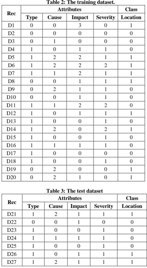
The incident instances are in multiples of hundreds, but for this study, the first 27 records, split into training dataset (table 2) and test dataset (table 3) are selected. The dataset has categorical attributes only, with small numbers of values – suitable for decision tree applications. The attribute values are coded (0,1,2,3,4 etc) as shown in the table 1.
No validation set is required. No missing values found in the selected dataset.
[image:2.595.313.558.74.518.2]The dataset is divided in a random proportion of 70:30 or 2/3:1/3 - ratio tested and proven to have produced the best result [10].
Table 1: Attribute values and codes for the incident dataset
Type:
0 -Potential/Near miss 1- With Consequence
Cause:
0 – Human error 1 – Equipment failure 2 – Sabotage/Theft
Impact:
0 – People 1 – Asset 2 – Environment 3 – Reputation
Severity:
0 – None 1 – Slight/Minor 2 – Major/Massive
Location:
0 – East (+) 1 – West (-)
Table 2: The training dataset.
Rec Attributes Class
Type Cause Impact Severity Location
D1 0 0 3 0 1
D2 0 0 0 0 0
D3 0 1 0 0 0
D4 1 0 1 1 0
D5 1 2 2 1 1
D6 1 2 2 2 1
D7 1 1 2 1 1
D8 0 0 1 1 1
D9 0 2 1 1 0
D10 0 0 1 1 0
D11 1 1 2 2 0
D12 1 0 1 1 1
D13 1 0 0 1 0
D14 1 2 0 2 1
D15 1 0 0 1 0
D16 1 1 1 1 0
D17 1 0 0 0 0
D18 1 0 0 1 0
D19 0 2 0 0 1
D20 0 2 1 0 1
Table 3: The test dataset
Rec Attributes Class
Type Cause Impact Severity Location
D21 1 2 1 1 1
D22 0 0 1 0 0
D23 1 0 0 1 0
D24 1 1 1 1 0
D25 1 0 0 1 0
D26 1 0 1 1 1
D27 1 2 1 1 1
The dataset has only two classes (representing the two branches of the Company) - East and West, coded as 0 and 1. The classes are also represented as + (for East) and – (for West) for simplicity of the tree diagram.
The training set is used for building the decision tree (called the classifier). The classifier is what is used to predict the classification for the instances in the test set .
4.BUILDING THE DECISION TREE
The method used is by applying the Entropy formula:From the training dataset (table 2):
Number of instances for the class Location = 0 is 11, Number of instances for class Location =1 is 9 and Total number of instances N (11 +9) is 20
Therefore Entropy (E) = -11/20*log2 (11/20) – 9/20*log2
The first step is to find the nodes and leaves of the decision tree. This is done by splitting process [12]. The splitting is practically done in levels - levels 1, 2, 3, etc. Each of the attribute is considered in each level.
4.1 Level 1 splitting:
Level 1 splitting process determines the root node. This is done by selecting the best attribute and performing a split on it [5]. Entropy and Gain is calculated for each of the attributes (type, Cause, Impact and Severity) to select the best-fit one.
(a).
Calculating Entropy and Gain for attribute
Type
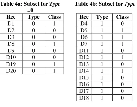
[image:3.595.54.276.221.393.2]Simply sort the training dataset with type, and then split into subsets Type = 0 and Type = 1, as in tables 4a and 4b.
Table 4a: Subset for Type =0
Table 4b: Subset for Type =1.
Rec Type Class
D1 0 1
D2 0 0
D3 0 0
D8 0 1
D9 0 0
D10 0 0
D19 0 1
D20 0 1
Rec Type Class
D4 1 0
D5 1 1
D6 1 1
D7 1 1
D11 1 0
D12 1 1
D13 1 0
D14 1 1
D15 1 0
D16 1 0
D17 1 0
D18 1 0
The Entropy for the subsets are:
For Type = 0: E0 = -4/8*log2 (4/8) – 4/8*log2 (4/8) = 1.0000
For Type = 1: E1 = -7/12*log2 (7/12) – 5/12*log2 (5/12) =
0.9799
Therefore, the Entropy for type is:
Etype = n/Σn*E0 + n/Σn*E1
= 8/20* 1.0000 + 12/20* 0.9799 = 0.9879, and the Information Gain is:
Gaintype = E - Etype
= 0.9928 - 0.9879 = 0.0049 The result of this calculation is as in table 4c.
Table 4c: Result of Entropy and Gain calculations for Type.
Type N East West E n/Σn*E
0 8 4 4 1.0000 0.4000
1 12 7 5 0.9799 0.5879
20 13 7 0.9879
Then E = 0.400 + 0.5879 = 0.9879, and Gain = 0.9928 - 0.9879 = 0.0049
Then the tree diagram for type is as in figure 3.
(b). Calculating Entropy and Gain for other attributes Cause, Impact, Severity will give:
Cause: E = 0.7979, Gain = 0.1949 Impact: E = 0.8316, Gain = 0.1612 Severity: E = 0.9578, Gain = 0.0350
The best-fit attribute is the attribute that leads to the split of maximal reduction of impurity i.e. lowest Entropy and highest Information gain, and it is Cause. Thus the root node is Cause.
4.2 Level 2 Splitting.
Level 2 splitting involves splitting the root node - Cause. The first task is to determine positions of the remaining attributes (Type, Impact and Severity) i.e. which one comes first and which one follows. The steps also involve recursive finding the minimal entropy (i.e. maximal information gain) of each.
From the dataset generated in level 1 operation:
Cause = 0, N = 10 (7+, 3-), therefore E= 0.8813 Cause = 1, N = 4 (3+, 1-), therefore E = 0.8113 Cause = 2, N = 6 (1+, 5-), therefore E = 0.6500
(a). Calculating the Entropy and Gain for attributes Cause = 0, Cause = 1 and Cause = 2
Following same steps as in level 1 above, the result of the class sorting (for determining the number of the class values) and the entropy of each class value are calculated and stated in tables 5a to 5i.
Note: Entropy alone is used to determine the best attribute. Gain is dropped since it is inverse proportional.
Table 5a: Entropy Calculation for Type on Cause =0.
Type N East West E
0 4 2 2 1.0000
1 6 5 1 0.6500
10 7 3
E = 0.7900
Table 5b: Entropy Calculation for Impact on Cause =0.
Impact N East West E
0 5 5 0 0
1 4 2 2 1.0000
2 0 0 0 0
3 1 0 1 0
10 7 3
E = 0.4000
Table 5c:Entropy Calculation for Severity on Cause =0.
Severity N East West E
0 3 2 1 0.9183
1 7 5 2 0.8631
2 0 0 0 0
10 7 3
E = 0.8797
Table 5d: Entropy Calculation for Type on Cause =1.
E = 0.6887
Type N East West E
0 1 1 0 0
1 3 2 1 0.9183
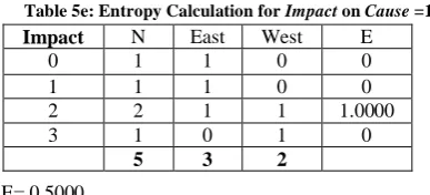
Table 5e: Entropy Calculation for Impact on Cause =1.
E= 0.5000
Impact N East West E
0 1 1 0 0
1 1 1 0 0
2 2 1 1 1.0000
3 1 0 1 0
5 3 2
Table 5f: Entropy Calculation for Severity on Cause =1.
Severity N East West E
0 1 1 0 0
1 2 1 1 1.0000
2 1 1 0 0
4 3 1
E = 0.5000
Table 5g: Entropy Calculation for Type on Cause =2.
Type N East West E
0 3 1 2 0.9183
1 3 0 3 0
6 1 5
E = 0.4591
Table 5h: Entropy Calculation for Impact on Cause =2.
E = 0.3333
Impact N East West E
0 2 0 2 0
1 2 1 1 1.0000
2 2 0 2 0
3 0 0 0 0
6 1 6
Table 5i: Entropy Calculation for Severity on Cause =2.
Severity N East West E
0 2 0 2 0
1 2 1 1 1.0000
2 2 0 2 0
6 1 5
[image:4.595.56.532.71.624.2]E = 0.3333
Table 5j: Summary for Entropy Calculation for Cause attributes.
Test
Attribute Entropy Values
Cause Type Impact Severity
0 0.7900 0.4000 0.8797
1 0.6887 0.5000 0.5000
2 0.4591 0.3333 0.3333
Table 5j is the summary of results for the three runs (cause = 0,1 and 2). Note that once an attribute is selected in a run, it is not considered for selection in the next run. The Bold typed figures (lowest entropy value, i.e. if not selected in the previous run) show attributes selected.
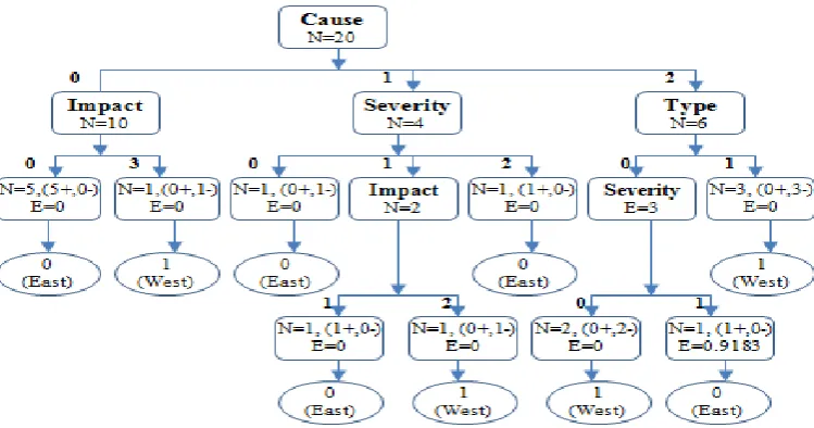
The tree diagram so far, for Cause = 0 (Impact), for Cause = 1 (Severity) and Cause = 2 (Type) is shown in figure 2.
4.3 Level 3 Splitting:
Splitting node A (i.e. cause =2, Type=0), the records that match node A are D9, D19 and D20, and the best-fit attribute (as in table 2) is Severity.
Splitting node B (i.e. cause =1, Severity =1), the records that match node B are D7 and D16, and the best-fit attribute (as in table 2) is Impact.
From the tree above, the nodes C, B and A are yet to get to the terminal (leaf) nodes because:
the attribute’s entropy is yet to be zero,
the samples in each node does not belong to the same class
there are more attributes on which the samples may be further partitioned.
[image:4.595.65.259.72.160.2] [image:4.595.65.509.439.620.2]Splitting node C (i.e. cause =0, Impact=1), the records that match node C are D4, D8, D10 and D12 and the best-fit (as in table 2) attribute is Type. The attribute type (for Cause = 0 and Impact = 1) is inconsistent. The equal subset numbers and entropy values are equal to 1 and do not make sense. In this case the attribute is said to have clashed and canbe subjected to Pruning and Overfitting [7]. The na node is not applicable too and is discarded.
Pruning helps to trim down the branches of the tree in a way that improves the generalization capability of the decision tree [6][13]. In decision tree, there are many ways of dealing with inconsistency or clashes, but the two principal ones are:
1. The “delete branch strategy” - where the branch with the clash is completely discarded and thus removing the instances from the training set.
2. The “majority voting strategy” - where the node with the more instances is taken, discarding the one with much less instances.
Applying option 1 above, the overall tree diagram is therefore is shown in figure 3.
5. EXTRACTING RULES FROM THE
GENERATED TREE
To generate rules (the model or classifier.), each path in the tree is traced - from root node to leaf node, recording the test outcomes as antecedents and the leaf-node classification as the consequent [5].
i.e IF antecedent(s) THEN consequent
Therefore the rules from the tree are as shown in figure 4:
R1: IF Cause = 0 AND Impact = 0 THEN Location = 0 R2: IF Cause =0 AND Impact =3 THEN Location = 1 R3: IF Cause = 1 AND Severity = 0 THEN Location = 0
R4: IF Cause = 1 AND Severity = 1 AND Impact = 1 THEN Location = 0 R5: IF Cause = 1 AND Severity = 1 AND Impact = 2 THEN Location = 1 R6: IF Cause = 1 AND Severity = 2 THEN Location = 0
R7: IF Cause = 2 AND Type = 0 AND severity = 0 THEN Location = 1 R8: IF Cause = 2 AND Type = 0 AND severity = 1 THEN Location = 0 R9: IF Cause = 2 AND Type = 1 THEN Location = 1
Figure 4: Decision tree rules/model.
6.
EVALUATING THE ACCURACY OF
THE MODEL
Many techniques are used to measure the performance of a model. Some require considerable amount of computation than others. Some require substantial more training instances to give reliable results [8]. Common among them are Re-substitution, Holdout, Cross-validation and Confusion matrix. As a matter of fact, there is no method that satisfies all constraints [10].
The methods used here for evaluating the accuracy of the derived model are the Holdout and Confusion Matrix methods.
6.1 Holdout Method
Testing the accuracy of the 9 rules on the 7 test records using Holdout method are as following:
Record D21 is correctly classified by R9 Record D22 is misclassified
Record D23 is correctly classified by R1 Record D24 is correctly classified by R4 Record D25 is correctly classified by R1 Record D26 is misclassified
Record D27 is correctly classified by R9
Thus 5 records out of 7 records are correctly classified, and the predictive accuracy is:
% 43 . 71 7 5
records tested of No
classified correctly records
of No Accuracy Predictive
or
Thus Error Rate = 2/7 or 28.57%
6.2 Confusion Matrix Method
[image:5.595.102.477.76.273.2]Table 6: Actual/predicted classification table. Class Actual Predicted Classified D21 1 Negative Negative correct D22 0 Positive Negative Error D23 0 Positive Positive correct D24 0 Positive Positive correct D25 0 Positive Positive correct D26 1 Negative Positive Error D27 1 Negative Negative correct
The confusion matrix for the test dataset is shown in table 7
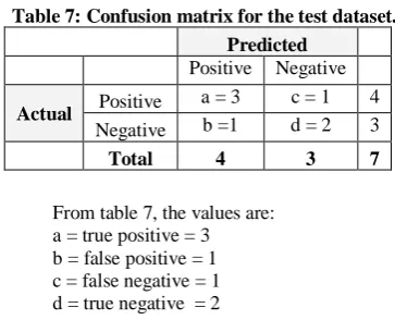
Table 7: Confusion matrix for the test dataset.
Predicted
Positive Negative
Actual Positive a = 3 c = 1 4 Negative b =1 d = 2 3
Total 4 3 7
From table 7, the values are: a = true positive = 3 b = false positive = 1 c = false negative = 1 d = true negative = 2
And the derived values therefore are:
N = a + b + c + d (the test sample size) = 7 Accuracy (Efficiency = (a + d)/N = 5/7 = 0.71 = 71.42%
Misclassification Rate = (b + c)/N = 2/7 = 0.28 = 28.57%
7. TESTING THE DECISION TREE
MODEL
Here, the derived model is tested with any other record form the incident database. This is done by manually plugging the attribute set of the unknown record into the derived model to see if the results would make sense.
Now test this:
If faced with an unknown situation with the attribute set Type = 1, Cause =1, Impact = 1 and Severity = 1, what would be the value of the class (location)?
Cross- checking the set of rules in figure 4, the rule that fits the attribute set is R4, which is (IF Cause = 1 AND Severity = 1 AND Impact = 1 THEN Location = 0)
This is interpreted as “if an incident with consequence (1) occur in the company, as a result ofequipment failure (1), with impact mainly on asset/property (1), and with Slight/Minorseverity(1), then the place the incident is likely to occur is in the east (0) location of the company”. This practically makes sense.
8. CONCLUSION AND
RECOMMENDATIONS
Industry safety dataset with its peculiar nature is successfully mined using decision tree classification tool. The perfect tree diagram (with very minimal overfitting) generated, in addition to the high accuracy rate of the model evaluation, prove that the DT tool is fit for the purpose.
The result of this investigation practically demonstrated that the decision makers of the company can quickly know ahead where and how to mobilise safety resources, make budgets and how to put barriers and controls to checkmate accidents. Even though this study came out with high accuracy rate, it is recommended that the further work still be carried out as it was observed that two or more equally accurate DT models can give different predictions. Hence it is worth examining the difference in accuracy of the two models, by applying some statistical tests such as confidence intervaland variance of observed deviation. To do this, it will require running a number of tests with other techniques to get the varying error rates. This area is not fully covered in this paper and it is worth practically investigating.
The accuracy of the predicted results may not always be high especially if inconsistent values (e.g. noise) and missing values, which are common to most real-live data, are found in the dataset. Hence datasets with inconsistence and missing values are worth trying.
Finally, pruning prevents tree from becoming so detailed but it memorizes the chance relationships in the developmental dataset instead of focusing on robust relationships that will carry over into independent data. Estimating the forecast error of the split’s leaves, estimating the forecast error of the pruned branch and deciding whether the split provides any worthwhile skill increase, are other better ways of managing overfitting and are recommended for further practical investigation.
9.REFERENCES
[1] Pang-Ning Tan, Michael Steinbach, Vipin Kumar, 2006, Introduction to Data Mining, Addison-Wesley Companion Books.
[2] Abbott D.W, Matkovsky P.I and Elder J.F, 1998, An
Evaluation of High-end Data Mining Tools for Fraud Detection, IEEE International Conference on Systems, Man, and Cybernetics, San Diego, CA, October 12-14,
1998. Paper download:
http://datamininglab.com/Portals/0/tool%20eval%20artic les/smc98_abbott_mat_eld.pdf
[3] Kurt Thearling, 2007, White Paper: An Introduction to Data Mining: Discovering hidden value in your data warehouse,
[http://www.thearling.com/text/dmwhite/dmwhite.htm]
[4] Gentle J.E, Hardle W, Mori Y, 2004, Handbook of Computational Statistics, Springer Edition, ISBN 10-3540404643.
[5] Alsabti K, Ranka S, and Singh V, August 1998. CLOUDS: Decision Tree Classification for Large Database. In Proceeding of 4th Intl. Conf. on Knowledge Discovery on Data Mining. New York, NY,
[7] Edelstein, Herbert A. 1999, Introduction to Data Mining and Knowledge Discovery, Third Edition. Potomac, Two Crows Corporation
[8] Jiawei Han, Micheline Kamber, 2006, Data Mining: Concepts and Techniques, The Morgan Kaufmann Series in Data Management Systems, ISBN 558609016.
[9] Ian H. Witten, Eibe Frank, Mark A. Hall; Data Mining, 2011, Practical Machine Learning Tools and Techniques (3rd Edition) Morgan Kaufmann, ISBN 978-0-12-374856-0
[10]Mitchell T, 1997, Decision Tree Learning: Machine Learning, The McGraw-Hill Companies, Inc.
[11]J. Ross Quinlan, 1975, Machine Learning, vol. 1, no 1.
[12]Hand D.J, Manila H, Smyth P, 2001, Principles of Data Mining, MIT Press
[13]Galit S, Nitin R. P, Peter C.B, 2010, Data Mining for Business Intelligence: Concepts, Techniques and Applications in Microsoft Office Excel with XLMiner, 2nd Edition, John Wiley & Sons, Inc. New Jersey, ISBN 978-0-470-52682-8.