Munich Personal RePEc Archive
Compressed Air Network Calculus Using
Computer Program
Dosa, Ion
University of Petrosani
2005
Online at
https://mpra.ub.uni-muenchen.de/62620/
SCIENTIFIC BULLETIN
OF THE POLITEHNICA UNIVERSITY OF TIMISOARA
Transactions on MECHANICS
Tom 51 (65) Fascicola 1, 2006
COMPRESSED AIR NETWORK CALCULUS USING COMPUTER
PROGRAM
Ion DOSA
University of Petrosani-ROMANIA, e-mail: [email protected]
Abstract: This paper presents the results obtained in developing a computer program for the calculus of compressed air networks
Key words: Compressed air network, computer program, exergetic balance
1. Introduction
The equations of gas dynamics are equations of balance. They permit to describe mathematically the gas flow through pipelines. The solutions for these equations applied to compressed air networks in case of the flow with friction, heat transfer and flow loss, can be obtained merely using numerical methods. These methods require a great volume of calculus. In case of compressed air networks, this becomes a problem, because the network has a great number of pipelines, embranchments, rings, elbows and fixtures. Therefore, the calculus of complex networks can be done only if the development of a computer program is considered.
The case of a mining compressed air network is studied, which by reason of his complexity, represents a special case of compressed air network.
Constructive peculiarities for such networks [1]: - Developing as the mine site evolves. Therefore the length of the network, his structure and the gas flow is constantly changing. The network structure became more complicated with lots of rings, rings with common edges, and all these alternating with embranchments.
- Must follow the mine works, resulting elbows, deviations and multiple embranchments.
- The ducts can t be welded, so the pipelines must be joined through flanges, therefore the flow losses can t be eliminated.
- The maximum length of pipelines that can be entered in underground is 6 m, a great number of joints resulting; therefore the flow losses are high.
- There are hard exploitation conditions. The pipelines and fixtures can be damaged, so that the
local pressure drops and the flow losses will grow. The corrosion of the pipelines is marked, which leads to the growth of the rugosity.
2. Mathematical model of compressed air network
Developing the mathematical model of compressed air networks, must start from the definition of his functional role, settlement of his limits, identification of its components and the relations that exist between these.
The compressed air network must be able to transport the compressed air from the compressor to consumers assuring the optimum operation parameters for these.
The limits of the system are represented through the outlet section of the buffer reservoir (compressors with piston) or the outlet section of the last cooler (turbocompressors) representing the inlet section of the network, the inlet section of the consumers representing the outlet section of the network and the lateral area of the pipelines.
The compressed air flows from the compressor through the inlet section of the network toward the consumer (through the outlet section of the network) with friction, heat transfer and flow loss through lateral area of the pipelines.
The discreet components of the compressed air network from the point of view of this analysis are [2], [3]:
- Fittings used for modification of the section of flow, changing the direction of flow and the
realization of the necessary embranchments.
- Fixtures that allow and direct the compressed air flow through pipelines, and also might adjust the parameters of the compressed air.
- Assembling parts that assure the connecting of components of the compressed air network.
Joining of these elements and their location in ground defines the structure of the compressed air network.
For modeling the structure of the compressed air network the representation of network as ordinary graph with the property that the maximum number of adjacent of a node is 4, is proposed.
According to the nodes of the graph different type of nodes of the network were defined:
- Compressor node corresponding to the compressor (or an injection point in the network) with the property that has only one adjacent;
- Embranchment node corresponding to the embranchments of network, can have 3 or 4 adjacent. - Consumer node - corresponding to the pneumatic consumer, can have only one adjacent.
Transom of the compressed air network, was defined as the physical succession of the discreet components of the network lined up between two nodes and corresponds the edges defined by two nodes in the ordinary graph.
The compressed air pipeline was defined as the succession of ducts joined through one of the known methods (flanged, welded, etc.) having the same diameter, lined up between two discreet components (section lift, faucets, diaphragms etc.)
Conclusively, the mathematical model of the compressed air network shall have two components:
- The algorithm of determination the structure of network, that describes the relations between different elements, the way of go through and the succession of calculus for the parameters of flow through the discreet elements of the network.
- Mathematical models for the calculus of parameters of compressed air flow through the elements of the network like: pipelines, faucets, elbows, flaps, valves, diaphragms, embranchments etc.
3. Mathematical model of air flow
The analytic determination of parameters of the compressed air flow through pipelines is possible through solving of the fundamental equations of gas dynamics singularized for compressed air networks.
Starting from the equations of gas dynamics applied to compressed air networks [4]:
- The continuity equation:
d 4 p d a = dx w) d( 2 1.3 ⋅ ⋅ ⋅ ⋅ π ρ (1)
- The momentum equation:
d 2 w -dx dp 1 -g = dx dw w 2
x ⋅ ⋅ ⋅
⋅ λ
ρ (2)
- The energy equation:
) T -(T c d w K 4 = dx dT m p ⋅ ⋅ ⋅ ⋅ ⋅ ρ (3)
- Equation of state: T R =
p ρ⋅ ⋅ (4)
relations in which: w is the average speed in section [m≅s-1], T - fluid temperature [K], Tm -surrounding
temperature [K], p fluid pressure [N≅m-2], d hydraulic diameter of the duct [m], density of the fluid [kg≅m-3], friction coefficient, K global heat transfer coefficient [W≅m-2≅K-1], a flow loss coefficient through leakiness.
From the relations (1), (2), (3), (4) above [4]:
) T R B -T w R -w g + w (A T R -w 1 = w x 3
2 ⋅ ⋅ ⋅ ⋅ ⋅ ⋅ ′ ⋅ ⋅ρ ' (5) ) T R + g -w A -w (B T R -w 1
= 2 x
2 ⋅ ⋅ ⋅ ⋅ρ⋅ ⋅ρ ⋅ρ⋅ ′
ρ'
In which A and B:
d p a 4 = B ; d 2 = A 1,3 ⋅ ⋅ ⋅ ⋅ π λ
The coefficients having the sign - for the calculus of transoms in the sense of fluid flow and the sign + for the calculus in opposite direction of fluid flow.
work [4] is recommended the use of the cubical spleen functions for the approximation of the solution of differential equations, due to the convergence of the method and steps of iteration that have relatively big values.
Also the losses through the fixtures of the compressed air network must be determinate because they enter different local resistances in the network. Because the value of the local resistance depends on the regime of fluid flow and the distribution of velocity in the flow section, the analytic determination of coefficients is often difficult. The researches showed as, in case of operations of the compressed air network in nominal regime, the flow through pipelines and hoses is turbulent in the quadratic area [10], and the relations of coefficients of local loss can be determined according to that assumption.
The values of local resistances determined experimentally are often given through tables or diagrams, and for different works [2], [3], [10], [11], these values can be more or less different. These differences appear in the case of formulae and suggested interpolation, too. From point of view of the mathematical model the way of tabular presentation or diagramms is disadvantageos, therefore on the strenght of these is recommended the use of the regression functions defined appropriately. The use of these functions simplifies many of the calculus of local resistances, because is obtained a relation that permits the direct calculus of the resistances depending on known parameters. In order to develop a complete and complex mathematical model, the data found in different works [2], [3], [10], [11] were remaked, so that analytic equations were defined for most of the local resistances found in mining compressed air networks.
These functions can be improved, by adding new data points, obtained from measurements, and finally will result a fairly approximation of the value of local resistances.
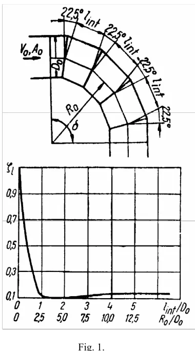
To illustrate the algorithm, is presented the result obtained for the elbow welded together from 5 elements with angles 22.5º (fig. 1).
The relation for the determination of the total resistance proposed in work [10] is:
d l 1) -(n + k k
= int
l
Re⋅ ⋅ ⋅ ⋅
Δ ζ λ
ζ (6)
where k is correctness coefficient for rugosity, kRe-
correctness coefficient for Re criteria, - friction coefficient, lint intermediate length between two
components [m], d hydraulic diameter [m], l
local resistance coefficient.
Comparing fig. 2 in which is represented the regressive function obtained on base of the data given in table 1 with the diagram presented in fig.1, is noticed the same form of the diagram, and the value of the coefficient of correlation R2=0.99 indicates the fact that between the two variables exist a strong correlation, therefore the function can be used to go on, not to mention that is simple to work with comparing to equation (6).
4. Algorithm for determination of network structure
[image:4.595.334.524.334.676.2]For simple network configurations, exists a big variety of calculation procedures, their complexity grow up as possibility of automate calculus improved, and especially along with the appearance of the electronic computers.
Fig. 1.
Table 1 R0/D0 l R0/D0 l R0/D0 l
0,5 0,75 2,5 0,12 12,5 0.14 0,98 0,45 5 0,10 15 0,14 1,47 0,34 7,5 0,12
1,9 0,15 10 0,14
Fig. 2.
Among first calculation procedures counted the one applied of acad. M.M. Fedorov [12] in which is considered the variation of the state of the compressed air flow in pipelines. The state of parameters of the air in any portion of the pipeline is determined in function of initial state parameters from the beginning of the pipeline.
The calculus of the network started from the compressor station toward to consumers.
The compressed air network can be projected choosing percentage of loss of pressure depending on value of admissible loss, so is obtained a minimum for the costs of the pipeline and the energy.
Acad. A.P. Gherman proposes the calculus of treelike networks from the consumer towards compressor [12].
In this case the pressure to consumers is the same, and is necessary the equalization of loss of pressure along of the branches that are not part of their nodes.
In behold of a computer program realization an algorithm [4] was developed, that require the division of some transoms with invariable geometric parameters in supplementary sectors, in order to obtain iterations with identical number of steps. Known parameters are: the configuration of the network, the length of the transoms, the demand of air input for the consumers, the temperature and the pressure of the compressed air at the outlet of the compressor station, the polytropic exponent of the
flow on the transom. Parameters resulting from calculus: loss of pressure on transoms, loss of flow on transoms, losses at the consumers, temperature on transom.
There are calculation procedures for treelike networks fed from one source, from two sources, for simple ring networks, and ring networks with common edges, for which the algorithms are depicted in the works [2], [53].
All these methods have a great disadvantage; they can be applied to networks with known configuration and in a differentiated way. The compressed air networks from underground are the result of the development in time of the mining works, have a complicated configuration, many branches and rings in different zones of the network.
Conclusively, an algorithm for compressed air networks must assure the way of go through the network in the sight of calculus and the identification of different sort of configurations.
Developing the algorithm for the calculus of the compressed air networks due to open with choosing the point from which the calculus began. According as, there are two possibilities: to go from the compressor to consumer, which presupposes a great number of iterations, and going from the consumer to compressor.
The second variant was chosen due to the fact that mathematical model permits the determination of transom parameters calculating from opposite direction of flow, and the number of iterations will decrease.
Is reminded as, the compressed air network is represented as an ordinary graph [13], [14], and in this case the calculus presupposes going in depth of the structure of graph, until to reach the consumer node.
Having in sight that a direct method of calculus doesn t exists, due to the complexity of the problem, a method that shall solve the problem through partial solutions must be found.
Such method is the Backtracking [13], in which the solution were build progressively.
Application of the method assumes the definition of static stacks which in shall kept the visited nodes and which will be erased only after the nodes are solved.
An embranchment node can be solved if known at least n-1 flows where n represent the number of adjacent.
strength of the flows and geometric sizes of the embranchment the resistance [10] and the missing pressure can be found, in assumption that the temperature is the same in all branches.
The ordinary graph defined through the nodes of the network and the proper transoms, is represented in the shape of a list of adjacent in a database.
Although exist another solution of representation [13], the choice was made since there are no limitations regarding the number of nodes, from the computer memory size point of view.
In the computer memory stood at one time solely the nodes visited and unsolved.
For the description of the algorithm of determination what nodes belong to a ring, have to start up from the definition [15], [16] of strongly connected graph, bi-connected graph and chain.
A limited chain which leaves from one point and comes back in the same point defines a ring.
The way of go through applied, assures that all the nodes in the graph will be visited.
Is noticed as, if we have rings with common transoms (edges), we have a lot of rings in the same structure, therefore many different roads from point v to point w, and although at one moment the return is happening in a node with visited neighbors, not all the nodes visited an unsolved shall belong to the same ring.
From the definition of the bi-connected component of the graph results as, any ring represents a connected component, and any bi-connected component is due to have at least one ring, where through once eliminated one node, exists a chain between any among the remnant nodes.
Therefore, the first step in the determination of the structure of the network is the determination of the bi-connected components of the subgraph defined by the visited nodes.
The algorithm for the determination of the bi-connected components of the graph is depicted in the work [13].
The determination of the rings from the bi-connected subgraph can be achieved using the algorithm of minimum distance in graphs [13], modified for the concrete established conditions through the definition of the subgraph, and applied repetitively until the subgraph has no more nodes that are not included in rings.
The results obtained using the algorithms presented therein before can followed using the computer program named REEA (NETWORK), which has an option that permits in depth visiting of
the graph nodes and the identification of ring components of a graph (compressed air network).
5. Results obtained, conclusions
The first analysis of the problem revealed, that in case of the compressed air network, the description of the nodes and transoms, the geometrical characteristics of different elements like ducts, elbows, faucets, fixtures etc., a great amount of data is used. Therefore programming language that can use large databases must be used to develop the program.
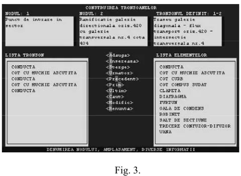
[image:6.595.303.543.472.647.2]The program [1] was developed to work with different networks. The main menu contains options for creating or deleting compressed air networks. Once a network created, can be opened to enter initial data, or to accomplish modifications or perform calculus. The first step is the input of data used for the description of the structure. Choose from the menu Reea (Network) the option Structur reea (Network structure) and type in the nodes, and the adjacent. The nodes can be labeled to distinguish easily between them. The transoms can be labeled too. If the network has a big number of nodes and transoms, this possibility of labeling is proved to be very useful when searching one of them. The program has, for all windows of data input, functions that validate the correctness of data entered. Also, for avoiding the start of calculus of a network with wrong or absent data, a menu for data validation was provided.
Fig. 3.
Fig. 4.
The menu is conceived so that doesn t permit the selection of an option until all the necessary conditions for data consistency were accomplished. The modification of network structure can be done selecting from the menu Reea (Network) the option Modificri structur (Structure modification), which offers the possibility of changing the labels of nodes and transoms, to erase them, adding or deleting adjacent. These operations must be made with special attention, for instance erase of a node leads to the deletion of all transoms that this node defines. If the network structure is correctly defined, the generation of transoms shall be done automatically, selecting the option from the menu Reea (Network). After the transoms were generated, the following option can be selected to carry out the construction of a transom from discreet elements.
This can be done easily, as noticed in fig. 3, in the right side of the screen exist a list of available elements, from which is chosen the desirable element, and choosing from the menu from middle the desirable option, the element can be added or inserted in the list of existing elements from the left side of the screen.
This makes building a transom very easy, any modification of elements from the transom can be done rapidly, without affecting other data. The order of elements of the transom in the list must be the same as found in ground, starting from the first node, toward the second. To the head of the screen were displayed the nodes that define the transom along with their labels.
In the menu Date iniiale (Initial data) can be selected an option only after the transom is validated with the help of the proper function, using the menu Validri (Data validations). With help of this menu the necessary initial data needed for calculus is
entered. In fig. 4 is presented the menu used for introduction of initial data for nodes.
Fig. 5.
After the initial data input and validation of these, calculus can start from the menu Calcule (Calculus) in which were three options Parcurgere fr calcule (Inspecting the network), Calcul (Calculus), Optimizare reea (Network optimization).
[image:7.595.333.512.120.326.2]For a selected option, on the screen shall be displayed permanently the results of calculus, respectively the visited node or transom and the results obtained for every element. After finishing the calculus, the results can be visualized selecting options from menu Rezultate (Results).
Fig. 6.
[image:7.595.330.515.513.675.2]of the exergetic balance of network, on sorts of loss, and the exergy lost on each type of network element: pipelines, diaphragms, elbows etc.
Fig. 7.
Fig. 8.
[image:8.595.307.539.298.496.2]The menu Erori (Errors) permits the visualization of error log files created with validation functions.
Fig. 9.
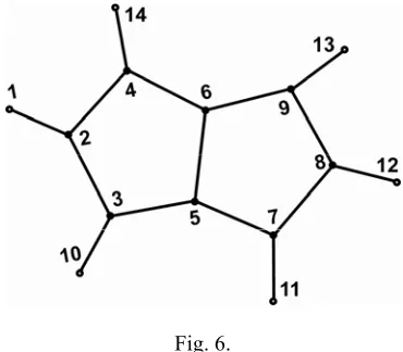
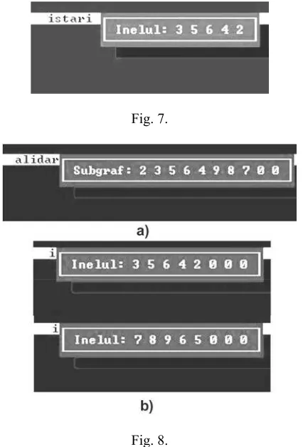
For verification of algorithms a ring shaped network fig. 5 and a network with two rings having a common edge fig. 6 were considered. After defining these, from menu Calcule (Calculus) choose Parcurgere fr calcule (Visiting nodes). The results obtained were represented in fig. 7 and fig. 8.
As seen, according to description of algorithm of go through, in case of the second network, first the subgraph containing the both rings were obtained fig. 8 a, and after that the two rings were separated fig. 8 b. The program was tested using data obtained through measurements [1] on a portion of compressed air network presented in fig. 9.
The calculus performed by the program permitted the drawing of the Sankey diagram from fig. 10.
Fig. 10.
Besides the data can be visualized with help of menu Rezultate (Results), (namely: parameters of state, losses, resistances, etc.), selecting the option Bilan exergetic (Exergetic balance) exergetic balance of network, can be visualized.
For the given network can be noticed that the greatest exergy loss is registered in pipelines and hoses (through friction and leakiness). Losses due to local resistances are smaller besides the loss from hoses and pipelines. Analyzing the losses of exergy by sorts can notice that the greatest loss registered is through leakiness, then through friction. The exergetic efficiency of transportation of the compressed air on network is 68.95%. The accuracy of determination the exergetic balance is 1.52%.
[image:8.595.54.291.515.704.2]solved. The program assures the recognition of most complex network configuration, so that after the calculus reaches to an end, data for any element of the network (faucets, elbows, etc.) can be found: initial parameters, final parameters, resistances, exergy losses or any other parameter compliant of mathematical model. The program has a big flexibility and simplicity regarding the use of great amount of data related to network, such as: the modification of a component of the network, erase of nodes and transoms, finding results, two-fold data validation once to introduction an then, before the beginning of calculus, in order to decrease to minimum the possibility of wrong data input, modular building that assures an easy development, through the modification of existing functions, or adding new functions.
References
1. Dosa, I.: Cercetri privind energetica proceselor termofluidodinamice din instalaiile pneumatice miniere (Research concerning thermo-fluid-dynamics processes from the pneumatic mining installations). IN: Doctoral dissertation, 1998, p.134-176, Petrosani. 2. Burducea, C., Leca, A.: Conducte i reele termice (Pipelines and thermal networks). IN: Editura Tehnic, 1974, Bucharest.
3. Leca, A., Priscaru, I., Tnase, H.M., Lupescu, L., Raica, C.: Conducte pentru ageni termici (Pipelines for thermal agents). IN: Editura Tehnic, 1986, Bucharest.
4. Irimie, I. I., Matei, I.: Gazodinamica reelelor pneumatice (Gas dynamics of pneumatic networks). IN: Editura Tehnic, 1994, Bucharest.
5. Dodescu, Gh., Toma, E.: Metode de calcul numeric (Numerical calculation procedures). IN: Editura Didactic i Pedagogic, 1976, Bucharest. 6. Larionescu, D.: Metode numerice (Numerical methods). IN: Editura Tehnic, 1989, Bucharest. 7. Rosculet, M.: Analiz matematic (Mathematical analysis). IN: Editura Didactic i Pedagogic, 1984, Bucharest.
8. Salvadori, M.G., Baron, L.M.: Metode numerice în tehnic (Numerical methods in technics). IN: Editura Tehnic, 1972, Bucharest.
9. Simionescu, I.: Metode numerice în tehnic Aplicaii în FORTRAN (Numerical methods in technics Applications in FORTRAN). IN: Editura Tehnic, 1995, Bucharest.
10. Idlecik, I.E.: Îndrumtor pentru calculul rezistenelor hidraulice (Guide for the calculus of
hydraulic resistances). IN: Editura Tehnic, 1984, Bucharest.
11. Kiselev, P.G.: Îndreptar pentru calcule hidraulice (Guide for hydraulic calculus). IN: Editura Tehnic, 1988, Bucharest.
12. Ilicev, A.C.: Instalaii pneumatice miniere (Pneumatic mining installations). IN: Editura Tehnic, 1951, Bucharest.
13. Cristea, V., Athanasiu, I., Kalisz, E., Iorga, V.: Tehnici de programare ( Techniques of programming). IN: Editura Teora, 1993, Bucharest. 14. Ionescu Texe, C., Zsako, I.: Structuri arborescente cu aplicaiile lor (Arborescent structures with their applications). IN: Editura Tehnic, 1990, Bucharest.
15. Cosoroab, C.: Compresoare cu piston (Compressors with pistons). IN: Editura Tehnic, 1964, Bucharest.
16. Vrânceanu, Gh., Gh., Mititelu, t.: Probleme de cercetare operaional (Problems of operational research). IN: Editura Tehnic, 1984, Bucharest.
CALCULUL REŢELELOR DE AER
COMPRIMAT UTILIZÂND UN PROGRAM DE CALCULATOR