A Firewall Application Using Binary Decision Diagram

2017 2nd International Conference on Computer, Network Security and Communication Engineering (CNSCE 2017) ISBN: 978-1-60595-439-4

A Firewall Application Using Binary Decision Diagram

Jun-feng ZHAO

, Yuan-yi XIA

and

Gao-jian LV

1

State Grid Jiangsu Information & Telecommunication Company, Nanjing, Jiangsu, China

2

List Youzu Interactive CO. LTD., Shanghai, China

Keywords: Firewall, Bdd, Redundancy removal.

Abstract. In this paper, we present our work on the application of the binary decision diagram (BDD) on the design of firewalls. We use the BDD as the underlying data. BDD is used to do the redundancy removal of firewalls. The basic idea is inspired by [1], the authors describe two kinds of redundant rules, respectively called “upward redundant rules” and “downward redundant rules”. Extensive experiments show that it is more efficient and more scalable by using bdd to do redundancy removal than using FDD.

Introduction

Firewalls are safety-critical systems that secure most private networks. Serving as the first line of defense against malicious attacks and unauthorized traffic, firewalls are crucial elements in securing the private networks of most businesses, institutions, and even home networks. A firewall is placed at the point of entry between a private network and the outside Internet so that all incoming and outgoing packets have to pass through it. Redundancy in firewalls is popular, and the removal of them is of vital importance.

Binary decision diagrams (BDDs) are extensively used in CAD (Computer Aided Design) software to synthesize circuits (logic synthesis) and in formal verification. We use in this paper BBD to remove redundancy of firewalls. Our implementation is built upon a BDD package called CUDD [2]. CUDD package provides a lot of basic procedure for manipulating BDDs. It also provides a wide range of variable reordering algorithms.

Related Work. In [3], the authors discussed how to use BDD to represent firewalls. In [6], the authors also used bdd to build a toolkit called “Fireman”. The problem of detecting redundant rules received attention in [1, 2, 4, 6, 7].

In [1], the authors gave a necessary and sufficient condition for identifying all redundant rules, based on which they categorize redundant rules into upward redundant rules and downward redundant rules. The authors presented methods for detecting the two types of redundant rules respectively by making use of a tree representation of firewalls. The BDD redundancy removal also based on the same idea. However, the underlying data structure is different, thus we can make use of the extensively studied binary decision diagram to do the redundancy removal. At least, this is another alternative to deal with the problem, and experiments show that BDD redundancy removal is more scalable and generally more efficient than FDD redundancy removal. To the best of our knowledge, this is the first work to use bdd in firewall redundancy removal

Binary Decision Diagram. A binary decision diagram (BDD), like a negation normal form (NNF) or a propositional directed acyclic graph (PDAG), is a data structure that is used to represent a Boolean function. For example the boolean expression (x1 ∨ x2) ∧ x3 can be represented by the

Figure 1. A simple decision diagram for (x1 ∨x2) ∧ x3.

A Boolean function can be represented as a rooted, directed, acyclic graph, which consists of decision nodes and two terminal nodes called 0-terminal and 1-terminal. Each decision node is labeled by a Boolean variable and has two child nodes called low child and high child. The edge froma node to a low (high) child represents an assignment of the variable to 0 (1). Such a BDD is called “ordered” if different variables appear in the same order on all paths from the root. It is called “reduced” if the graph is reduced according to two rules:

(a) Merge any isomorphic subgraphs.

(b) Eliminate any node whose two children are isomorphic.

In popular usage, the term BDD almost always refers to Reduced Ordered Binary Decision Diagram (ROBDD in the literature, used when the ordering and reduction aspects need to be emphasized). The advantage of an ROBDD is that it is canonical (unique) for a particular functionality. This property makes it useful in functional equivalence checking and other operations like functional technology mapping. A path from the root node to the 1-terminal represents a (possibly partial) variable assignment for which the represented Boolean function is true. As the path descends to a low child (high child) from a node, then that node’s variable is assigned to 0 (1).

Our Work. The motivation to use BDD instead of FDD to deal with firewall is due to the following consideration. First, BDD is extensively studied for decades. Some basic procedure like

and, or and not is implemented very efficiently. Moreover, there exists a lot of reordering algorithms

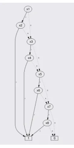
Figure 2. Good variable ordering.

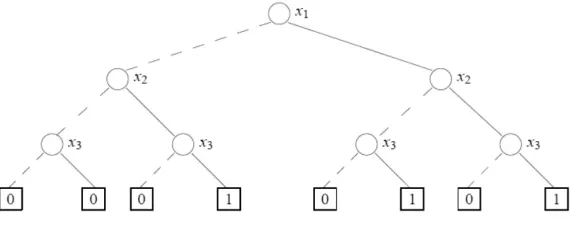
Regarding the importance of variable reordering, simply put, if we have a boolean function f(x1, . .

., xn) then depending upon the ordering of the variables we would end up getting a graph whose

number of nodes would be linear at the best and exponential at the worst case. For example, let us consider the Boolean function f(x1, . . . , x2n) =x1x2 + x3x4 + . . . + x2n−1x2n. Using the variable ordering

x1 < x3 < . . . < x2n−1 < x2 < x4 < . . . < x2n, the BDD needs 2n+1 nodes to represent the function. Using

the ordering x1 < x2 < x3 < x4 < . . . < x2n−1 < x2n, the BDD consists of 2n nodes. These two different

ordering are shown in Figure 3 and Figure 2.

Figure 3. Bad variable ordering.

Redundancy Removal Using BDD

In this conversion, we also record the mapping information. This is a one-to-many mapping, i.e., one firewall rule maps to one or multiple binary format rules. Second, we convert every binary rule into a BDD. This step is straightforward, i.e., one variable is assigned to denote every bit. In our implementation, it costs 105 variables to denote a binary format rule. After that, we do upward redundancy removal and downward redundancy removal respectively. In these two redundancy removal steps, we detect all redundant binary format rules. Finally, we compute the original redundancy with the knowledge of redundant binary format rules and the mapping information computed in the first step.

Changing a Rule into Binary Format. Due to the nature of BDD, our approach first converts firewall rules from original format into binary format. Be more specific, we convert one original rule into one or multiple prefix rules. In our experiment, we check the following five fields for every firewall rule: source IP address, destination IP address, source port number, destination port number, and protocol type. The length of these packet fields are 32, 32, 16, 16, and 8 respectively. Another one bit is used to denote the decision. So every binary rules has the length of 105. Because in the real firewall, a port field sometimes may be denoted by an interval. For a 16 bits interval, in the worst case, it requires 30 different prefixes to denote it. Thus, in the worst case, one original rule will be mapped to at most 900 rules.

In binary rules, we use “1”, “0” and “*”. “*” matches both “1” and “0”. For example, a port number 25 will be converted to its 16 bits binary format: 0000 0000 0001 1001. A port range 0-65535 will be converted to **** **** ********.

While converting a firewall into binary format, the mapping information is stored. Basically we use bdd redundancy removal program to detect all the redundant binary format rules. After that, we can detect the original firewall’s redundancy by examining the mapping info.

Converting Every Binary Format Rule into a BDD. Every binary format rule consists of 104 bits predicate and 1 bit decision. One variable is assigned to each bit of predicate. Variables are stated in explicit order to build a BDD.

Upward Redundancy Removal. For upward redundancy removal, we have the following Theorem:

Theorem 1 One rule is upward redundant if and only if its predicate is totally matched by its

previous rules. In other words, the resolving set of that rule is empty.

In the following pseudocode, we used a CuddBddOr procedure to union two bdds. CuddBddLeq is used to check whether one bdd is implied by another BDD. CuddBddAnd is used to compute the common part of two bdds. CuddNot calculates the compliment of a bdd.

Upward Redundancy Removal Algorithm

Input : Corresponding BDD for every binary format rules, b[1..n]

Output: Redundancy flag list, redundant[1..n] Rules resolving set, resolving[1..n]

Steps: for i := 1 to n

redundant[i] = false;

Build an empty BDD called ball for i := 1 to n

if(CuddBddLeq(b[i], ball))

set redundant[i] = true;

else

set redundant[i] = false;

resolving[i] = CuddBDDAnd(b[i], CuddNot(ball))

ball = CuddBddOr(b[i], ball)

End

Theorem 2 Let f be any firewall that consists of n rules:<r1, r2,… , rn>. Let b'_i (2 ≤ i≤n) be an BDD that is equivalent to the sequence of rules <ri, ri+1, ··· , rn>. The rule ri−1 with the effective rule set Ei−1

is downward redundant in f iff the effective rule set Ei−1’s corresponding bdd is contained in b'_i.

Downward Redundancy Removal Algorithm

Input : Corresponding BDD for every binary format rules, b[1..n]

Every binary format rule’s decision decision[1..n]

Rules resolving set, resolving[1..n]

Previous redundancy flag list computed in upward redundancy removal, redundant[1..n]

Output: Final Redundancy flag list, redundant[1..n]

Steps:

1. Build an empty BDD called ball 2. for i := n to 1

if(redundant[i] == false)

if(decision[i] == accept)

if(CuddBddLeq(resolving[i], ball))

redundant[i] = true;

else

ball = CuddBddOr(b[i], ball);

else

resolving[i] = CuddNot(resolving[i]);

btmp = CuddNot(b[i]);

if(CuddBddLeq(ball, resolving[i]))

redundant[i] = true; else

ball = CuddBddAnd(btmp, ball);

End

Computing Redundancy for the Original Firewall. We have detected all binary redundant rules during upward and downward redundancy removal. We also have the mapping info which denotes the relationship between original rules and binary format rules. We can compute the redundancy for the original firewall through the following procedure.

Compute Redundancy for Original Firewall Algorithm

Input : mapping[1..m], in which stores the number of binary rules for each original rule.m is the number of original rules. backMapping[1..n], in which stores the corresponding original rule number for each binary format rule. n is the number of binary format rules. redundancy flag list computed in upward and downward redundancy removal, redundant[1..n] Output: Final Redundancy flag list, finalredundant[1..m]

Steps:

for i := 1 to m

finalredundant[i] = false;

for i := 1 to n

if (redundant[i] == true)

let t = backmapping[i];

mapping[t] = mapping[t] − 1;

if (mapping[t] == 0)

finalredundant[t] = true;

Experimental Results

We have tested on both the implementation of FDD redundancy removal and BDD redundancy removal. First, we compare them on some real firewalls. Table 1 shows the comparison result.

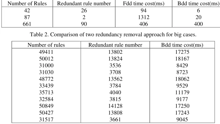
From statistics of Table 1, we noticed bdd approach is faster than fdd approach. Especially for the 87 rules case, using bdd is nearly 65 times faster than using fdd.

Table 1. Comparison of two redundancy removal approach for three real firewalls.

Number of Rules Redundant rule number Fdd time cost(ms) Bdd time cost(ms) 42 87 661 26 2 90 94 1312 406 6 20 400

Table 2. Comparison of two redundancy removal approach for big cases.

Number of rules Redundant rule number Bdd time cost(ms) 49411 50012 31000 31030 48772 33439 35713 32584 50849 50427 31517 13802 13824 3536 3708 13562 3784 4040 3815 14128 13808 3661 17275 18167 8429 8723 18062 9529 11179 9177 17250 17243 9045

We further tested some big firewalls on both implementations. Each of these test cases has more than 30000 rules. While the fdd implementation suffers from memory explosion, our bdd implementation can still compute out the result within 20 seconds. Table 2 shows the bdd redundancy removal statistics for these big cases.

From these test cases, we have seen that the bdd redundancy removal is not only faster but also more scalable than fdd redundancy removal.

Conclusions and Future Work

In this paper, we address a firewall problem by using BDD. We use BDD to do redundancy removal. Preliminary results show that this approach is very promising. From our experiments, we have seen that the bdd redundancy removal is not only faster but also more scalable than fdd redundancy removal.

Possible future work includes using bdd as the underlying structure to do firewall queries. Another thing is to extend the bdd procedures to deal with firewalls which have more than two decisions. We may also use bdd to do analysis for distributed firewalls.

References

[1] A. X. Liu and M. G. Gouda. Complete redundancy detection in firewalls. In Proceedings of 19th

Annual IFIP Conference on Data and Applications Security (DBSec-05), 196-209(2005).

[2] U. of Colorado at Boulder. Cu decision diagram package. In http://vlsi.colorado.edu/ fabio/CUDD/cuddIntro.html.

[3] A. F. Scott Hazelhurst and A. Henwood. Binary decision diagram representations of firewall and router access lists. In Technical Report TR-Wits-CS-1998-3. (1998).

[4] E. Al-Shaer and H. Hamed. Firewall policy advisor for anomaly detection and rule editing. In

[5] E. Al-Shaer and H. Hamed. Management and translation of filtering security policies. In IEEE

International Conference on Communications, pages 256–260. (2003).

[6] E. Al-Shaer and H. Hamed. Discovery of policy anomalies in distributed firewalls. In IEEE

INFOCOM, pages 2605–2616. (2004).

[7] P. Gupta. Algorithms for routing lookups and packet classification. In PhD thesis, Stanford