Stochastic modelling and equilibrium in mathematical finance and statistical sequential analysis

(1)

The London School of Economics and Political Science A thesis submitted to the Department of Mathematics

for the degree of Doctor of Philosophy

Stochastic modelling and equilibrium

in mathematical finance and statistical

sequential analysis

Author:

Yavor Stoev

Supervisors:

Dr. Pavel V. Gapeev Dr. Albina Danilova

(2)

Declaration

I certify that the thesis I have presented for examination for the MPhil/PhD degree of the

London School of Economics and Political Science is solely my own work other than where I

have clearly indicated that it is the work of others (in which case the extent of any work carried

out jointly by me and any other person is clearly identified in it).

The copyright of this thesis rests with the author. Quotation from it is permitted, provided

that full acknowledgement is made. This thesis may not be reproduced without my prior

written consent.

I warrant that this authorisation does not, to the best of my belief, infringe the rights of

any third party.

(3)

2

Abstract

The focus of this thesis are the equilibrium problem under derivative market imbalance, the

sequential analysis problems for some time-inhomogeneous diffusions and multidimensional

Wiener processes, and the first passage times of certain non-affine jump-diffusions.

First, we investigate the impact of imbalanced derivative markets - markets in which not all

agents hedge - on the underlying stock market. The availability of a closed-form representation

for the equilibrium stock price in the context of a complete (imbalanced) market with terminal

consumption allows us to study how this equilibrium outcome is affected by the risk aversion

of agents and the degree of imbalance. In particular, it is shown that the derivative imbalance

leads to significant changes in the equilibrium stock price process: volatility changes from

constant to local, while risk premia increase or decrease depending on the replicated contingent

claim, and become stochastic processes. Moreover, the model produces implied volatility smiles

consistent with empirical observations.

Secondly, we study the sequential hypothesis testing and quickest change-point (disorder)

detection problem with linear delay penalty costs for certain observable time-inhomogeneous

Gaussian diffusions and fractional Brownian motions. The method of proof consists of the

reduction of the initial problems into the associated optimal stopping problems for

one-dimensional time-inhomogeneous diffusion processes and the analysis of the associated free

boundary problems. We derive explicit estimates for the Bayesian risk functions and optimal

stopping boundaries for the associated weighted likelihood ratios and obtain their exact rates

of convergence under large time values.

Thirdly, we study the quickest change-point detection problems for the correlated

compo-nents of a multidimensional Wiener process changing their drift rates at certain random times.

These problems seek to determine the times of alarm which are as close as possible to the

unknown change-point (disorder) times at which some of the components have changed their

(4)

appropri-ate posterior probability processes exit certain regions restricted by the stopping boundaries.

We characterize the value functions and optimal boundaries as unique solutions of the

associ-ated free boundary problems for partial differential equations. We provide estimates for the

value functions and boundaries which are solutions to the appropriately constructed ordinary

differential free boundary problems.

Fourthly, we compute the Laplace transforms of the first times at which certain non-affine

one-dimensional jump-diffusion processes exit connected regions restricted by two constant

boundaries. The method of proof is based on the solution of the associated integro-differential

boundary problems for the corresponding value functions. We derive analytic expressions for the

Laplace transforms of the first exit times of the jump-diffusion processes driven by compound

Poisson processes with multi-exponential jumps. The results are illustrated on the constructed

non-affine pure jump analogues of the diffusion processes which represent closed-form solutions

of the appropriate stochastic differential equations.

Finally, we obtain closed-form expressions for the values of generalised Laplace transforms

of the first times at which two-dimensional jump-diffusion processes exit from regions formed by

constant boundaries. It is assumed that the processes form the models of stochastic volatility

with independent driving Brownian motions and independent compound Poisson processes

with exponentially distributed jumps. The proof is based on the solution to the equivalent

boundary-value problems for partial integro-differential operators. We illustrate our results

in the examples of Stein and Stein, Heston, and other jump analogues of stochastic volatility

(5)

4

Introduction

I.

Description of the subject

The main themes of this thesis are the equilibrium problem in mathematical finance under

derivative market imbalance, the sequential analysis problems of mathematical statistics and

the first passage times of non-affine jump-diffusions driven by solvable equations.

The question of how the market of financial derivatives impacts the underlying asset prices

in equilibrium plays an important role in financial economics and mathematical finance. With

the current market of over-the-counter derivatives having outstanding notional amount of more

than ten times that of the world stock market, it is crucial to understand the potential impact

trading in such contracts can have on the stock prices. In standard frictionless (complete)

models of financial markets the introduction of structured financial products does not have an

influence on asset prices in equilibrium - this is due to the fact that derivatives are assumed

to be in zero net supply and long positions can be offset by taking the corresponding short

ones. In reality, however, a lot of the counterparties in such contracts do not hedge them or do

so only infrequently. Effectively, the market in the underlying asset becomes imbalanced - an

extra supply or demand is created which could potentially impact the dynamics of asset prices.

Apart from the intuitive considerations, there has been number of studies supporting the

idea that hedging has an effect on market risk premia and volatility (see e.g. Basak [6] and

Grossman and Zhou [49]). The event that triggered investigations into the impact of dynamic

hedging strategies was the market crash of 1987. The rise of the so-called portfolio insurance

strategies, which guarantee a minimum level of wealth at some horizon, together with

auto-mated trading in the years surrounding the crash, led researchers to study them as a possible

cause for the high volatility during the crash. Moreover, after the crash the implied volatility

started exhibiting the now characteristic smile, suggesting that the Black-Scholes model may

(8)

on the magnitude and direction of the market impact and our main motivation here is to

pro-vide a general setting which can account for both increasing/decreasing risk premia and market

volatilities.

In practice, in order to be able to find the equilibrium stock prices in the above problem, we

need to have some externally given quantities (e.g. the dividend growth rate of the underlying

asset) that we have estimated through statistical methods. However, no agent has perfect

information - the dividends contain noise and the growth rate can change without the agent

realizing it. Nevertheless we have to rely on observable data, as it arrives, in order to infer the

true value - this is a problem of statistical sequential analysis.

Sequential analysis problems are concerned with the analysis of data that doesn’t have a

fixed sample size. These problems were initially used in improving industrial quality control

but later numerous applications were found in many real-world systems in which the amount

of observation data is increasing over time (see, e.g. Carlstein et al. [20] for an overview). Two

of the classical problems of this type are the sequential hypothesis testing and quickest

change-point (disorder) detection. In the sequential hypothesis testing problem the aim is to determine

the true value, among two alternatives, for the parameter of some observable quantity. The

problem was first studied for sequences of independent and identically distributed observations

by Wald and Wolfowitz [115, 116]. The problem of quickest change-point detection seeks to

determine a stopping time which is as close as possible to the time of change-point at which the

observable quantity changes its probabilistic properties. Originating from the control charts

introduced by Shewhart [100], different variants of the problem were subsequently developed

(see Page [84]).

In both of the sequential analysis problems described above one faces a tradeoff between

min-imizing the observation time and the error due to noise in the observations. The usual method

of solving these problems, as developed in Mikhalevich [79] and Shiryaev [101, 102, 103, 104],

is to reduce them to optimal stopping problems for Markov processes called sufficient

statis-tics, and then prove verification theorems that characterize the value functions and optimal

stopping boundaries as unique solutions to free boundary problems for ordinary or partial

(integro-)differential operators. In order to carry out the verification arguments additional

conditions are imposed, which guarantee the uniqueness of the solution of the free boundary

problem. The smooth-fit condition was seen to hold for the value functions when the

underly-ing sufficient statistics can leave the continuation region determined by the optimal stoppunderly-ing

(9)

as-I. Description of the subject 8

sociated optimal stopping theory can be found in the books of Shiryaev [105] and Peskir and

Shiryaev [90].

The link between optimal stopping and free boundary problems led to the availability of

analytic expressions for the solutions of the sequential analysis problems. Nevertheless, even for

simple model specifications (e.g. when the observable is one-dimensional Brownian motion with

changing/unknown constant drift), finding explicit solutions to the associated free boundary

problems is nontrivial and additional relations between the model parameters are often assumed.

Thus, one is often lead to search for estimates of the original value functions and optimal

stopping times, which are easier to compute. Our aim here is to provide verification theorems

and estimates in new and more general models for the observable processes.

Stochastic processes representing solutions to stochastic differential equations are used in

modelling phenomena that exhibit random behaviour. Therefore, in the theory of stochastic

differential equations, it is important to have analytical tractability of the resulting models. A

lot of problems in these models become computationally feasible if probabilistic properties of

the related stochastic processes, such as the probability densities or characteristic functions of

their marginal distributions, have closed-form expressions. Well-known examples can be found,

beginning with the seminal work of Bach´elier [5], where he constructed a discrete pre-image

of Brownian motion for the description of the stock prices on a financial market, in Ornstein

and Uhlenbeck [112], where the authors used a mean-reverting process to study velocity of a

massive particle in a fluid under the bombardment by molecules, and in the geometric Brownian

motion proposed by Samuelson [97] for modelling the behavior of financial assets. A recently

popularized general class of tractable models, for which the form of the characteristic function

is known, are the affine processes (see Duffie et al. [33]). An alternative class of continuous

processes that can be used in modelling, and which can be non-affine, are those that satisfy

solvable stochastic differential equations. These equations can be solved explicitly as shown in Gard [45; Chapter IV] or can be reduced to first-order ordinary differential equations as in

Øksendal [83; Chapter V], and thus provide tractability of the resulting models. Another form

of model tractability comes from the ability to compute the Laplace transforms of the first

passage times of a stochastic process - these are the times at which the process crosses given

values. Knowledge of the Laplace transform of the first passage times gives rise to numerous

applications in engineering (e.g. see Blake and Lindsey [17]) and mathematical finance (see Kou

and Wang [68]). Our objective in the final part of the thesis is to obtain analytic expressions

(10)

solving stochastic differential equations, which contain jumps and are extensions of the solvable

class, as well as for certain jump analogues of stochastic volatility models.

II.

Historical notes and references

We present here historical notes and references to the relevant literature on the problems solved

in this thesis, by also pointing out the position of our results.

The problem of finding equilibrium on the market is central in economic theory and has

received a lot of attention in mathematical finance recently. The essence of equilibrium is to

regard the asset prices as results of the aggregate trading decisions of rational agents on the

market, that bring the supply and demand in balance. Starting from microeconomic principles

one usually works with agents which have concave preferences, maximize expected consumption

and possess exogenously given income streams (i.e. endowments).

The concept of an economy in equilibrium, by looking at prices as a result of supply and

demand forces, was introduced in Walras [117]. For the first time existence of equilibrium was

proved in a static mathematical framework containing several agents and commodities by

Ar-row and Debreu [4]. The earlier equilibrium models were in discrete-time and extending them

to continuous-time introduced an infinite dimensional problem. This difficulty was overcome

in Karatzas et al. [61, 62, 59] in a continuous-time complete market setting. There the

au-thors present the now standard method of finding equilibrium, by using results from portfolio

optimization (see Karatzas et al. [60]) together with a finite-dimensional fixed point argument

first introduced in Negishi [81]. Numerous extensions to the above classical setting has been

considered - see Karatzas and Shreve [64; Chapter 4] for an overview.

The study of equilibrium with agents that are not pure utility maximizers was motivated

by the emergence of the volatility smile effect after the market crash of 1987 and the possible

influence that dynamic hedging strategies had on the stock price volatility (see Grossman

[47], Grossman and Villa [48] ). In Brennan and Schwarz [18] the effect of portfolio insuring

on the equilibrium stock prices was investigated. The final wealth of a portfolio insurer was

given by a fixed terminal payoff containing an implicit put option on a proportion of the

total market wealth. This lead to increase in market risk premium and (implied) volatilities.

Portfolio insurers were modelled as final wealth utility maximizers having lower bound on wealth

in Grossman and Zhou [49]. Existence of equilibrium prices was proved for logarithmic and

(11)

II. Historical notes and references 10

magnitude of change in market quantities like volatilities and risk premia in different market

states, they provided evidence that market volatility increases. In a related setting Basak [6]

proved existence of equilibrium where the portfolio insurers maximized CRRA utility from

consumption, and had insurance horizon which ended before the terminal market date. The

conclusion was that the market price of risk level stays the same, while the volatility decreases

due to the presence of portfolio insurers, which hinted at the importance of the specification

of agent’s utilities and the market investment horizon (see also Basak [7] for an alternative

modelling of the agents’ utilities).

In equilibrium literature the completeness of the market is often assumed to hold apriori.

However it is more desirable to obtain a complete market as an outcome of equilibrium, which

gives rise to the notion endogenous completeness. Recently a series of papers concentrated in proving endogenous completeness of equilibrium - see Anderson and Raimondo [2], Hugonnier

et al. [52], Riedel and Hirzberg [94] and Kramkov and Predoiu [70]. The key assumptions in

the above articles are the Markov property of the model primitives (e.g. dividends or market

factors) as well as the real analyticity of the exogenous volatility. In Chapter 1 we prove the

existence of equilibrium and its endogenous completeness in a setting where not all agents

hedge - i.e. some contingent claims are not in zero net supply and the market for them is

imbalanced. We achieve this effect by including a hedging agent in the market that acts as

a risk minimizer and wants to perfectly replicate a contingent claim underwritten to another

agent that is outside of the market and does not hedge. This is more in line with the definition

used in [18] and we have a clear separation of the risk-minimizing and the utility-maximizing

effects on the market prices.

The problems of statistical sequential analysis that we are interested in seek to determine

the distributional properties of continuously observable stochastic processes with minimal costs.

The problem of sequential testing for two simple hypotheses about the drift rate of an observable

Gaussian process is to detect the form of its drift rate from one of the two given alternatives.

In the Bayesian formulation of this problem, it is assumed that these alternatives have an a

priori given distribution. The problem of quickest change-point (disorder) detection for an

ob-servable Gaussian process is to find a stopping time of alarm τ which is as close as possible to the unknown time of change-point θ at which the local drift rate of the process changes from one form to another. In the classical Bayesian formulation, it is assumed that the random

(12)

identically distributed random variables (see, e.g. Shiryaev [105; Chapter IV, Sections 1,3]).

The first solutions of the problems in the continuous-time setting were obtained in the case

of observable Wiener processes with constant drift rates (see Shiryaev [105; Chapter IV,

Sec-tions 2 and 4]). The standard disorder problem for observable Poisson processes with unknown

intensities was introduced and solved in Davis [25], under certain restrictions on the model

parameters. Peskir and Shiryaev [88, 89] solved both sequential analysis problems for Poisson

processes in full generality (see also [90; Chapter VI, Sections 23 and 24]). The case of

observ-able compound Poisson processes, in which the unknown characteristics were the intensity and

distribution of jumps, was investigated in Dayanik and Sezer [27, 28]. Other formulations based

on the exponential delay penalty setting were studied in Beibel [12] for a Wiener process and

in Bayraktar and Dayanik [8] for a Poisson process. These problem settings are suitable when

modelling situations in which the costs of delay in disorder detection are not necessarily linear

and another measure of the error due to false alarms is preferable (e.g. continuous

compound-ing of interest rate in financial applications). The classical change-point detection problem for

Poisson processes for various types of probabilities of false alarm and delay penalty costs was

studied in Bayraktar et al. [9]. More general versions of the standard Poisson disorder problem

were solved by Bayraktar et al. [10], where the intensities of the observable processes changed

to unknown values. These problems for observable jump processes were solved by successive

approximations of the value functions of the corresponding optimal stopping problems. This

method was also applied in the solution of the disorder problem for observable Wiener process

in Sezer [99], in which disorder happens at one of the arrival times of an observable Poisson

process. Further extensions of both sequential analysis problems for observable Wiener

pro-cesses were studied in Gapeev and Peskir [41, 42] in the finite horizon setting, and for certain

time-homogeneous diffusions in Gapeev and Shiryaev [43, 44] on infinite time intervals.

In the classical infinite horizon setting for the observable Wiener processes explicit solutions

can be obtained, since the corresponding differential operator is an ordinary one. This fails

to hold in the finite horizon setting, because the corresponding partial differential operator

contains a time derivative. However, in the studies of more realistic models with non-stationary

increments, the equivalent free boundary problem becomes parabolic and no explicit solutions

exist in general, even in the infinite horizon case (see Chapter 2).

Multidimensional versions of the quickest disorder detection problems naturally arise when

one models real-world systems described by several stochastic processes which may have

(13)

II. Historical notes and references 12

independent Poisson processes, in which stopping times were sought as close as possible to the

minimum of the two disorder times. Dayanik et al. [26] solved the disorder problem for

ob-servable multidimensional Wiener and Poisson processes with independent components, which

change their local characteristics simultaneously. The quickest change-point detection problem

for observable multidimensional Wiener process with correlated components that change their local drift rates at different disorder times is studied in Chapter 3. Possible applications of the solutions of these quickest detection problems include: assembly line breakdown in plant

production of an item when we aim to detect the minimum of all disorder times (see [11]);

abnormal returns in one of many stocks when we aim to detect just one of the disorder times;

total system breakdown when we aim to detect the maximum of all disorder times.

The method of reducing stochastic differential equations to solvable ones was studied in

Gard [45; Chapter IV], where closed-form strong solutions to a class of stochastic differential

equations with linear coefficients were obtained, by introducing an integrating factor process.

The idea is further developed in Øksendal [83; Chapter V], for equations with general drift

coefficients, which are reduced to the ordinary differential form. Certain reducibility criteria

were provided in Gapeev [38] for diffusions driven by a Wiener process and a Poisson random

measure of a finite intensity. Jump analogues of continuous diffusions satisfying solvable

equa-tions were constructed and shown to have the same support of marginal distribuequa-tions as the

original processes, making them a suitable modelling alternative. The latter fact was justified

by Iyigunler et al. [54], where simulations studies were provided for this model.

An introduction to the topic of financial modelling with jump-diffusions is provided in

Runggaldier [96], where asset price and term structure models are studied in the context of

pricing and hedging. An extensive overview of L´evy process models with multiple numerical

and empirical examples is given in the book of Cont and Tankov [21]. The general class of affine

processes, which includes L´evy processes, was introduced in Duffie et al. [33]. The logarithm

of the characteristic function of these processes is affine in their initial value and is known in

an analytic form through a solution of a family of ordinary differential equations. This leads

to tractability of the resulting models and makes them suitable for applications to the

term-structure of interest rates (see [33; Chapter 13] and references therein), credit risk (see Duffie

[32]), stochastic volatility (see Kallsen [57]) and option pricing by Fourier methods (see e.g.

Kallsen et al. [58]). Despite the recent focus on affine processes, there are still models that fall

outside this general framework. Some well-known examples are the CEV and SABR models

(14)

calibration methods are known (see [50]). An overview of both affine and non-affine models for

interest rates can be found in Shiryaev [106; Chapter III, Section 4].

The Laplace transform of the first time to a given drawdown of a Brownian motion with

linear drift and the running maximum stopped at that time was computed by Taylor [110], and

the joint law of those variables was obtained by Lehoczky [74]. Some explicit expressions for

other related characteristics such as the expectation and the density of the maximum drawdown

of the Brownian motion with linear drift were derived by Douady, Shiryaev and Yor [31] and

Magdon-Ismail et al. [76], respectively. More recently, Sepp [98] derived closed-form expressions

for the Laplace transforms of the first hitting time of constant boundaries for double-exponential

jump-diffusion process. Mijatovi´c and Pistorius [78] obtained the laws of the first-passage times

of spectrally positive and negative L´evy processes over constant levels as well as analytically

explicit identities for a number of characteristics of drawdowns and drawups in those models.

III.

Contribution of the thesis

Let us now describe the contribution of the thesis to the problems of equilibrium, sequential

analysis and stochastic modelling described above.

We prove the existence of endogenous equilibrium in an imbalanced derivative market

(Chapter 1). We begin by specifying the financial market, which consists of a

(representa-tive) agent that maximizes utility from final wealth and a hedging agent that wants to exactly

replicate the payoff of a given contingent claim. There is a bond and a risky stock that

rep-resents a claim to a dividend at the final trading date. The dividend is the final value of an

exogenously given Markov process. We prove existence of an equilibrium stock price process

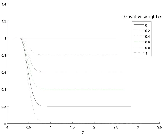
that makes the market complete, and provide its local volatility form for utilities having index

of relative risk aversion less than 1. This is in contrast with the constant volatility resulting

from classical equilibrium setting containing only power utility maximizers. By varying the

replicated contingent claim we can obtain any volatility smile shape. Thus we can explain

the presence of volatility smile by the presence of hedgers on the market, confirming one of

the explanations for the Black Monday market crash of 1987. In particular, in comparison to

the usual setting with only a representative agent, hedging strategies corresponding to long

positions in European options lead to higher implied volatility levels at their associated strike

(15)

III. Contribution of the thesis 14

In order to find the equilibrium stock price process we use results from portfolio

optimiza-tion in complete markets (see [60]), to obtain a guess for the state-price density. Indeed, if

equilibrium exists and the resulting market is complete, the hedger can replicate exactly the

contingent claim and, assuming zero initial wealth, his final wealth will be equal to the

con-tingent claim minus its arbitrage-free price. By market clearance we obtain the final wealth

of the utility-optimizing agent and we use duality results from Kramkov and Schachermayer

[71] to find the state-price density process as conditional expectation of the marginal utility

at the agent’s final wealth. Knowing the state-price density we can obtain the stock price

process again as conditional expectation of the terminal dividend. We find the arbitrage-free

price of the contingent claim as a solution to a fixed point problem. Finally, we prove that the

obtained guess for the stock price process results in complete market by using the recent result

on endogenous completeness in [70].

We consider the two classical problems of sequential analysis in their Bayesian

formula-tions for certain Gaussian processes with non-stationary increments (Chapter 2). We begin

by providing a unifying optimal stopping problem for the likelihood ratio processes, which are

time-inhomogeneous diffusions. This allows us to work with both original problems in a

con-sistent way. We prove a verification theorem and show that the optimal stopping times are the

first times at which the associated likelihood ratios exit from certain regions. Such regions are

restricted by the curved stopping boundaries, which are solutions to the equivalent parabolic

free boundary problems. Since we intend to provide an explicit analysis for the asymptotic rates

of the solutions, we introduce an auxiliary ordinary differential free boundary problem in which

the time variable is a parameter, by removing the time derivative from the initial parabolic

operator. The resulting ordinary differential equation admits an explicit solution, and we can

obtain closed-form estimates for the solutions of the original parabolic problem. We derive

analytic expressions for the optimal boundaries in the auxiliary problem, and specify their

ex-act asymptotic behaviour under large time values. Combining these results with the estimates

of the solutions of the original optimal stopping problem, we can check that the assumption

of the main verification theorem, that the optimal stopping time has finite expectation, is

in-deed satisfied. We demonstrate this in a setting in which the observable process is a fractional

Brownian motion with a constant drift rate. In that case we can reduce the sequential analysis

problems to the original unifying optimal stopping problem for time-inhomogeneous diffusion

processes.

(16)

multidi-mensional Wiener process (Chapter 3). This problem seeks to determine the times of alarm at

which some of the components of the process change their local drift rates as soon as possible

and with minimal error probabilities. The classical Bayesian formulation of these problems

con-sists of minimization of linear combinations of the probabilities of false alarm and the expected

linear penalty costs in detecting the change-points correctly. It is customary assumed that the

change-point (disorder) times are independent exponentially distributed random variables. Our

setting is closer to the one of [11], since the component disorder times are different, but is more

general in the sense that we observe multiple correlated components.

We begin by reducing the original disorder problem to an optimal stopping problem for a

multidimensional Markov diffusion. The components of the diffusion form a family of posterior

probability processes, corresponding to every subset of disorder times, and play the role of

sufficient statistics for the original disorder problem. When doing the reduction, we use the

ideas from [40], where the filtering equations for the posterior probabilities are derived for two

observable correlated Wiener processes. It is shown that the optimal stopping times are the

first times at which one of the posterior probability processes exits from a region restricted by a

stochastic boundary surface, determined by the current values of the other sufficient statistics.

We formulate the equivalent free boundary problem and prove a verification theorem that

identifies its unique solution with the value function of the optimal stopping problem. The

main complication in our setting arises from the higher dimensions of the sufficient statistics

needed to formulate the optimal stopping problem for a Markov process, due to the presence

of several disorder times. Moreover, the correlation structure of the observable processes has

to be taken into account when deriving the filtering equations. The proof of the verification

theorem uses the change-of-variable formula with local time on surfaces from Peskir [87]. As

we do not have explicit solutions to the free boundary problem, we provide lower estimates for

the value functions, which inherently construct the upper estimates for the stochastic boundary

surfaces, in the case in which we aim to detect the infimum of component disorder times. These

estimates are solutions to free boundary problems for ordinary differential equations.

We introduce an analytically tractable framework in which the Laplace transforms of

cer-tain exit times for non-affine jump analogues of continuous diffusion models can be computed

(Chapter 4). We begin by extending the method of [45; Chapter IV] for finding solvable

stochastic differential equations to a general class of jump-diffusions. By applying a smooth

invertible transformation, the original equation is reduced to a simpler one with linear diffusion

(17)

IV. Structure of the thesis 16

closed-form solutions. Moreover, we construct jump analogues of certain continuous diffusion

models driven by solvable equations, by following the method described in [38]. We provide

examples of reducing solvable equations and constructing their non-affine jump-diffusion

ana-logues for several popular models. Finally, we consider the first times at which non-affine jump

analogues of continuous diffusion models, with compensator measures correspond to compound

Poisson processes, exit from an open interval on the real line. We characterize the integrals of

the Laplace transforms of these exit times as solutions to ordinary differential boundary value

problems, by reducing the integro-differential equation corresponding to the original jump

ana-logue generator. Explicit solutions are provided for the pure jump anaana-logues of the CIR, CEV

and the nonlinear filter models with compensator measures corresponding to a compound

Pois-son process with one-sided exponentially distributed jumps.

We derive closed-form expressions for the generalised Laplace transforms of the first exit

times of the two-dimensional jump-diffusion processes from certain connected regions formed by

constant boundaries (Chapter 5). We consider two-dimensional jump-diffusion processes driven

by independent standard Brownian motions and independent compound Poisson processes

with exponential jumps. We provide closed-form solutions of the partial integro-differential

boundary-value problems associated with the values of the generalised Laplace transforms as

iterated stopping problems for the two-dimensional jump-diffusion processes forming the

mod-els of stochastic volatility. In particular, we derive closed-form expressions for the generalised

Laplace transforms in jump analogues of Stein and Stein and Heston as well as in other

stochas-tic volatility models.

IV.

Structure of the thesis

In Section 1.1 we specify our financial market and remark on some useful properties of the

exogenous Markov process that models the dividends. In Section 1.2 we prove the existence of

endogenously complete equilibrium and provide analytic expressions for the equilibrium stock

price drift and diffusion coefficients as well as the optimal portfolio of the representative agent.

Moreover we prove the local volatility form of the stock price process for certain utility functions.

Finally, in Section 1.3, we illustrate our results when the exogenous Markov process modelling

the dividends is of Black-Scholes type, and the representative agent maximizes power utility.

In this simple setting, we show the effect of the replicated contingent claim on the implied

(18)

In Section 2.1 we formulate a unifying optimal stopping problem for the time-inhomogeneous

diffusion likelihood ratio process and show how this problem arises from the Bayesian sequential

testing and quickest change-point detection settings. We formulate an equivalent free boundary

problem and derive explicit solutions of the auxiliary ordinary free boundary problems which

have the time variable as a parameter. In Section 2.2 we study the asymptotic behavior of

the resulting stopping boundaries under large time values, by means of deriving their Taylor

expansions with respect to the local drift rate of the observable process. In Section 2.3 we

apply these results to models with observable fractional Brownian motions by proving that the

optimal stopping times have finite expectations and, hence, the verification theorem can be

applied to characterize the solutions of the sequential analysis problems.

In Section 3.1 we introduce the setting of the model for the quickest change-point detection

problem for observable multidimensional Wiener processes. We derive stochastic differential

equations for a family of posterior probability processes corresponding to subsets of the disorder

times, by means of generalized Bayes’ formula (see [75; Theorem 7.23]). In Section 3.2 we

construct the associated optimal stopping problem for the posterior probability processes and

formulate the equivalent high-dimensional free boundary problem. The verification theorem

is proved providing characterization of the optimal stopping boundary surface as the unique

solution to the free boundary problem. Finally, in Section 3.3, we provide estimates for the

original solution to the problem of detection of the infimum of all disorder times.

In Section 4.1, we apply the method of [45; Chapter IV] to obtain explicit solutions to

jump-diffusion stochastic differential equations with linear coefficients. Then we follow [83;

Chapter V, Example 5.16] to reduce the equations with general drift and linear diffusion and

jump coefficients to ordinary differential equations that are satisfied pathwise (see also [38]). In

Section 4.2, we extend the class of solvable stochastic differential equations via smooth invertible

transformations, and provide sufficient conditions for their reducibility. We also construct jump

analogues of continuous diffusions and give some examples. In Section 4.3, we show that the

Laplace transforms of the first exit times from a region restricted by two constant boundaries for

certain finite activity pure jump analogues of continuous diffusions can be obtained by solving

ordinary differential equations, and provide explicit solutions for some popular models.

In Section 5.1, we first introduce the setting and notation of the model with a

two-dimensional jump-diffusion Markov process which has the price of the risky asset and the

volatility rate as the state space components. We define the generalised Laplace transforms of

(19)

V. Acknowledgments 18

Section 5.2, we obtain a closed-form solution to the partial integro-differential boundary-value

problem under several additional conditions on the parameters of the model. In Section 5.3,

we verify that the resulting solution to the boundary-value problem provides the joint Laplace

transform. The main results of the paper are stated in Theorem 5.3.1.

V.

Acknowledgments

First and foremost, I would like to thank my doctoral supervisors Dr. Pavel V. Gapeev and

Dr. Albina Danilova for the countless hours invested in mentoring and guiding me during my

doctoral studies at the London School of Economics, and for strengthening my knowledge in two

diverse subfields of stochastic analysis. Dr. Pavel V. Gapeev introduced me to the fascinating

topic of sequential analysis, shared his ideas and helped me in developing a solid understanding

of the subject, and improved my mathematical writing immensely. Dr. Albina Danilova helped

me in grasping the elegant idea of economic equilibrium and building a strong foundation in

portfolio optimization, and made my mathematical argumentation more rigorous.

I am thankful to the faculty members of the Department of Mathematics and the

Depart-ment of Statistics, and in particular to Dr. Christoph Czichowsky, Dr. Arne Lokka, Professor

Adam Ostaszewski, Dr. Hao Xing and Professor Mihail Zervos for the helpful

mathemati-cal discussions. I also want to thank the doctoral students in mathematimathemati-cal finance from the

Department of Mathematics at LSE with which I have spent a lot of time studying different

concepts in mathematical finance and stochastic analysis.

I would like to express my gratitude to the people that made administrative matters for a

doctoral student easy, namely Rebecca Lumb and Dave Scott.

I gratefully acknowledge the financial support of the Department of Mathematics without

which this doctoral thesis would not have been possible.

Last but not the least, I would like to thank my family for the constant support during my

(20)

Chapter 1

Equilibrium with imbalance of the

derivative market

This chapter is based on joint work with Dr. Albina Danilova.

1.1.

Financial market and model primitives

Let (Ω,F,_P) be a probability space rich enough to support a Brownian motion (Wt)t∈[0,T] and

let (Ft)t∈[0,T] be its filtration satisfying the usual conditions, where T ≥0 is a terminal time.

Consider a financial market consisting of two assets:

A riskless zero yield bond with maturity T and in total supply of K ∈_R units.

A risky asset, i.e. a stock with an adapted price process S = (St)t∈[0,T], which is in total

supply of 1 unit and represents a time T claim to an exogenously given random dividend.

Both assets are continuously traded on the time interval [0, T] and we assume that the market terminates after this time. Let the exogenously given log-dividend process Z = (Zt)t∈[0,T] be

the unique strong solution of the stochastic differential equation (SDE)

dZt =µZ(t, Zt)dt+σZ(t, Zt)dWt for t∈[0, T], (1.1.1)

with initial condition Z0 =z0 ∈R and some functions µZ(t, z) : [0, T]×R→R and σZ(t, z) :

[0, T]×_R →_R. Denote by Cb(R) the space of bounded and continuous real-valued functions

(21)

1.1. Financial market and model primitives 20

Assumption 1.1.1. The functions µZ(t, z) and σZ(t, z) satisfy the following conditions:

(C1) Uniform ellipticity: σ2

Z(t, z) is uniformly bounded away from zero, i.e. there exists σ >0

such that σ2

Z(t, z)≥σ on [0, T]×R.

(C2) Boundedness and analyticity: µZ(t, z) and σZ2(t, z) are bounded on [0, T]×R. The maps

t → µZ(t,·) and t → σZ(t,·) from [0, T] to Cb(R) are analytic on (0, T), i.e. for all

t ∈ (0, T) there is a constant ε(t) > 0 and sequences (An(t))n≥0, (Bn(t))n≥0 in Cb(R) such that

µZ(s,·) =

∞ X

n=0

An(t)(s−t)n and σZ(s,·) =

∞ X

n=0

Bn(t)(s−t)n,

for any s ∈(0, T) with |s−t|< ε(t).

(C3) Continuity: µZ(t, z) and σZ(t, z) are uniformly H¨older-continuous in t for all z ∈ R,

and σ2_Z(t, z) is uniformly H¨older-continuous in z for all t ∈ [0, T]. Moreover, µZ(t, z)

and σZ(t, z) are locally Lipschitz-continuous in z for all t∈[0, T].

Remark 1.1.1. From Theorems 5.3.11 and 5.3.7 in [35] we can see that (C2) and (C3) guar-antee the existence of a weak solution to (1.1.1)that is pathwise unique up to an explosion time. From the boundedness in (C2) we get that the explosion time is a.s. infinite (see Chapter IX, Exercise 2.10 in [93]) and therefore the solution is pathwise unique for all t ∈ [0, T]. From Theorem IV.1.1 in [53] it follows that there exists a unique strong solution to (1.1.1)with initial condition Z0 = z0 ∈ R. Moreover, for any (t, z) ∈ [0, T]×R, the SDE in (1.1.1) has unique

strong solution Z(t,z) _on _[_{t, T}_] _satisfying

P[Zt(t,z) =z] = 1.

We use conditions (C1)-(C3) to prove some properties of the marginal distributions of Z

(see Lemma 1.A.1 in the Appendix) and to obtain unique solutions to certain terminal value (Cauchy) problems with respect to the infinitesimal generator _LZ of (t, Zt)t∈[0,T]. Moreover, we

can apply Theorem 9.2 in [37] to obtain a fundamental solution (see Definition 5.7.9 in [63]) of the partial differential equation (PDE)

LZG(t, z) :=

∂G

∂t(t, z) +µZ(t, z) ∂G

∂z(t, z) +

σ_Z2(t, z) 2

∂2G

∂z2(t, z) = 0, (1.1.2)

for (t, z) ∈ [0, T)×_R. We denote this fundamental solution by p(t1, z;t2, v) where 0 ≤ t1 <

t2 ≤T and z, v ∈R.

(22)

nonzero a.e. a.s., which will lead to the endogenous completeness of the equilibrium market (see [69]).

Let us now specify the properties of the stock price processes on the market.

Definition 1.1.1. The stock price process S is admissible if the following conditions are sat-isfied:

S is a continuous, strictly positive semimartingale with absolutely continuous finite vari-ation part, meaning that it satisfies

dSt=St(µtdt+σtdWt) for t ∈[0, T], (1.1.3)

for some Ft-progressively measurable processes (µt)t∈[0,T] and (σt)t∈[0,T] such that

Z T

0

|µt|dt <∞,

Z T

0

σ2_tdt <∞, a.s..

The equality ST = exp(ZT) holds.

The market is complete, i.e. we have that Z T

0

µ2

t

σ2_tdt <∞, a.s.,

the process

exp−

Z t

0

µ2

s

σ2

s

dWs−

1 2

Z t

0

µ2

s

σ2

s

ds,

is a martingale and σt 6= 0 a.e. a.s..

Remark 1.1.2. It is known from Theorem 7.2 in [29] (see [65, 13] for more recent results) that the No Free Lunch with Vanishing Risk (NFLVR) property together with the local boundedness of the stock price process implies its semimartingality. This fact is used in [3] to show that the boundedness of an agent’s expected utility implies the NFLVR property, and therefore that the stock price is a semimartingale (see also [15, 73, 65]). The continuity of the stock price process is a consequence of its local martingality under some equivalent measure change and the fact that we work in a Brownian filtration. Therefore, the assumption that S is a continuous

1_{For a discussion as to why the conditions on the stock price process imply this representation, see [64;}

(23)

semimartingale is not too restrictive. Furthermore, the intuitive requirement that the stock price should be equal to the random dividend at time T, i.e. ST = exp(ZT), can be justified by the

fact that, otherwise, an obvious arbitrage opportunity exists and NFLVR is not satisfied. It is reasonable to expect that an admissible stock price processS leads to a complete financial market, since there is a single source of risk and an asset that allows agents to trade this risk. Our definition of a complete market follows the one of a standard market in Definition 1.5.1 in [64] together with the characterization of a complete market in Theorem 1.6.6 in [64].

There are two agents trading in the bond and the stock on the financial market – thehedger

and the optimizer. The agents differ in their endowments and portfolio optimization problems. The hedger wants to replicate a nontraded contingent claim h(ST), where h(z) : [0,∞) → R

is a payoff function. The optimizer has utility from final wealth u(z) : (0,∞)→_R and wants to maximize its expectation. In the following definition we specify the admissible portfolios on the market.

Definition 1.1.2. Let S be an admissible stock price process. An Ft-progressively measurable

process π = (πt)t∈[0,T] is called a self-financing portfolio process if we have

Z T

0

|πtµt|dt <∞ and

Z T

0

π2_tσ_t2dt <∞ a.s., (1.1.4)

and the corresponding wealth process Xπ = (X_tπ)t∈[0,T] satisfies

X_tπ =X₀π+

Z t

0

πudSu for t∈[0, T], (1.1.5)

for some initial wealth Xπ

0 ∈ R. We define the set Ab of all (self-financing) portfolios with

wealth processes that are bounded from below by a constant b ∈_R as

Ab

:=π is a self-financing portfolio process: X_tπ ≥b a.s. for t ∈[0, T] ,

and denote AB _:=S

b∈RA

b_{. The portfolio process} _π _{will be called admissible if} _π _{∈ A}B_.

We set the initial endowments (i.e. wealth) of the agents are zero for the hedger and S0+K

for the optimizer, respectively. The following conditions on the payoff h will be needed:

Assumption 1.1.2.

h(z) is a continuous function and there exist k, k >0 such that

h(z) = a1z+b1 for z ∈[0, k] and h(z) = a2z+b2 for z ≥k, (1.1.6)

(24)

h(z) is bounded from below, h6≡0, and the condition

h(z)< z+h0 for z >0, (1.1.7)

holds for some constant h0 ≥0. We have that h1 ≤K−h0 where

h1 := max

0,−min

z≥0 h(z)

. (1.1.8)

Remark 1.1.3. The assumption that h(z) is linear for small and large z allows us to prove integrability of certain expressions of the marginal utility (see Lemma 1.A.1 in the Appendix). The boundedness from below of h(z) guarantees that the hedger will be able to replicate the claim with an admissible portfolio.

We require that the upper bounds on h(z) and h1 hold, because they guarantee that the

optimizer has a strictly positive final wealth (see Theorem 1.2.1 below). One can easily see this in the case when the payoff h(z) is nonnegative, since then we have from (1.1.8) that K ≥h0

and, hence, condition (1.1.7)leads to ST+K > h(ST), i.e., the total endowment on the market,

which is initially held by the optimizer, is larger than the replicated claim by the hedger.

Let us precisely define the solutions to both agents’ problems.

Definition 1.1.3. Let S be an admissible stock price process.

1. The process π is a solution to the hedger’s problem if π is an admissible portfolio and the corresponding wealth process Xπ_{, with} _Xπ

0 = 0, satisfies XTπ = h(ST)−xh, where

xh _∈

R is the arbitrage-free price of the contingent claim h(ST) given by

xh =_E

h(ST) exp

−

Z T

0

µ2_t σ2

t

dWt−

1 2

Z T

0

µ2_t σ2

t

dt

. (1.1.9)

2. The process π is a solution to the optimizer’s problem if π is an admissible portfolio that solves the final wealth utility maximization problem

sup

π∈AE

[u(X_Tπ)],

where A := π ∈ A0 _:

E[min(0, u(XTπ))] > −∞ and the corresponding wealth process

(25)

Since we want the above utility maximization problem to be well-posed we introduce the

following set of assumptions:

Assumption 1.1.3.

u(z) is a strictly increasing, strictly concave, C2((0,∞)) function satisfying

lim

z→0+u

0

(z) = ∞, lim

z→∞u 0

(z) = 0 (Inada conditions). (1.1.10)

The asymptotic elasticity of u(z) is less than 1, meaning that

lim sup

z→∞

zu0(z)

u(z) <1. (1.1.11)

The index of relative risk aversion of u(z) is bounded, i.e.

−zu00(z)

u0₍_z₎ ≤R for z >0, (1.1.12)

for some constant R > 0.

Remark 1.1.4. We need the standard assumptions (1.1.10)-(1.1.11) on the utility function

u(z) in order to guarantee the existence of a unique solution to the optimizer’s problem. The condition (1.1.12) was used in [69] to prove the completeness of the financial market in equi-librium. In particular, from (1.1.12) we can see that the decreasing function logu0(ez₎ _has

derivative bounded from below by −R and, hence, there exists a constant N > 0 such that

lnu0(ez₎_{< N}_{(1 +}_|_z_|₎_{. It follows that (see also Lemma 6.1 in [69])}

u0(ez)≤eN(1+|z|), −u00(ez)≤R eN+(N+1)|z| for z >0. (1.1.13)

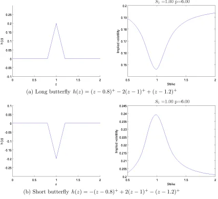
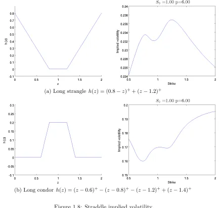
Example 1.1.5. Some payoff functions h(z) that satisfy the above conditions are bounded from below linear combinations of European call and put options, such that the sum of the coefficients in front of the call payoffs is at most 1, i.e.

h(z) =

n

X

i=1

αi(z−Ki)++βi(Ki−z)+,

where αi, βi ∈ R and

Pn

i=1αi ∈ [0,1] for n ∈ N. For the utility function u(z) we can take

u(z) = log(z) or u(z) = z1−p/(1−p) for p∈(0,1)∪(1,∞).

(26)

Definition 1.1.4. Equilibrium in the finite-horizon financial market is a process triple (S, πh_,

b

π)

such that the stock price process S is admissible, the processes πh _and

b

π solve the hedger’s and optimizer’s problems in Definition 1.1.3, respectively, and the following condition holds:

Clearing of the stock market:

πh+π_b= 1 λ([0, T])⊗_P a.e. a.s., (1.1.14)

where λ([0, T]) denotes the Lebesgue measure on the interval [0, T].

Since the wealth processes of both agents are of the form (1.1.5) and their initial wealth is

given, from the clearing of stock market condition it follows:

Clearing of the bond market:

Xh−πhS+Xb−πS_b =K λ([0, T])⊗P a.e. a.s., (1.1.15)

where we have denoted the hedger’s and optimizer’s wealth processes by Xh = (X_th)t∈[0,T] and

b

X = (Xb_t)_t∈[0,T] respectively.

Remark 1.1.6. Let us comment on the form of condition (1.1.15). The quantities Xh₋_πh_S

and Xb − b

πS on its left hand side correspond to the wealth of each agent that is invested in bonds. However, since the bonds have zero yield, these quantities also represent the number of bonds held by each agent. Since on the right hand side we have the total number of bonds on the market, the condition (1.1.15) indeed means that the bond market clears, i.e. the supply and demand of bonds are equal. In combination with (1.1.14) this also leads to the clearing of the whole market wealth, i.e. Xh₊

b

X =S+K a.e. a.s..

(27)

1.2. Main results 26

While our notion of equilibrium is the classical one, our model is nonstandard, as the market

contains an agent that does not maximize utility – the hedger. The introduction of a hedging

agent in the market allows us to study how equilibrium prices are affected when there are

derivatives which are not in zero net supply, as is the case with the contingent claim h(ST).

1.2.

Main results

In order to find the equilibrium stock price process S we use ideas from portfolio optimization in complete markets. We describe below the heuristic argument through which we obtain a

guess for the state-price density and, subsequently, the stock price process.

Suppose that equilibrium exists and the resulting market is complete. The hedger can

replicate exactly the contingent claim with final wealth given by Xh

T =h(ST)−xh, where the

constant xh _{is the arbitrage-free price of} _h₍_S

T). Since the market clears at time T, the final

wealth of the optimizer will be Xb_T = S_T +K −h(S_T) +xh. Now we can use duality results

(e.g. see Theorems 2.0 and 2.2 in [71]) to get that the state-price density process L at time T

is given by

LT =

u0(ST +K−h(ST) +xh)

E[u0(ST +K−h(ST) +xh)]

.

If, moreover, L is a martingale, we obtain L at any t ∈[0, T) as Lt=E[LT|Ft]. Thus we have

obtained a guess for the state-price density. Finally, if the process L S is a martingale (and not only a local martingale), we can obtain a guess for the stock price process St by taking

conditional expectation, i.e. LtSt =E[LTST|Ft] for any t∈[0, T).

After obtaining the guess for the stock price process S, what is left is to check that the resulting market is indeed complete and in equilibrium. However, for this line of reasoning

to work, we need to apriori specify the arbitrage-free price xh _{of the contingent claim} _h₍_S T),

which, by looking at the form of LT, should satisfy

xh =_E[h(ST)LT] = E

[h(ST)u0(ST +K−h(ST) +xh)]

E[u0(ST +K−h(ST) +xh)]

.

Let us first prove a lemma that gives the existence and uniqueness of a solution to the

equation for xh.

Lemma 1.2.1. Let Assumptions 1.1.1, 1.1.2 and 1.1.3 be satisfied. There exists a constant

xh ≥ −h1 satisfying

(28)

where xh _>₋_h

1 if h(z) is not a negative constant, and xh =−h1 otherwise. Moreover, if u(z)

satisfies

−zu00(z)

u0₍_z₎ ≤1 for z >0, (1.2.2)

then the equation (1.2.1) has a unique solution.

Proof. We begin by proving the existence of a solution in the interval [−h1,∞) via an

appli-cation of the intermediate value theorem.

Denote ξ(z) = (z−h(Z))u0(Z +K+z−h(Z)) for z ≥ −h1, where Z := exp(ZT). Since

K ≥h0+h1 and (1.1.7)-(1.1.8) hold, we have that Z+K+z−h(Z)>0 and ξ(z) is well-defined.

We will first prove that _E[ξ(z)] is a continuous function for z ≥ −h1. Choose z ≥ −h1 and

δ >0 and let z0 ∈[−h1, z+δ). Since u0(z) is decreasing and the conditions in (1.1.7)-(1.1.8)

are satisfied, we obtain

|ξ(z0)| ≤

z0−h(Z)

u0(Z +K +z0−h(Z))

≤(z+δ+ max(h1, h0+Z))u0(Z +h0−h(Z)).

From Lemma 1.A.1 in the Appendix we conclude that (z+δ+max(h1, h0+Z))u0(Z+h0−h(Z))

is an integrable random variable and we have by the dominated convergence theorem

lim

z→zE[ξ(z)] = E[limz→zξ(z)] = E[ξ(z)].

Hence _E[ξ(z)] is a continuous function for z ≥ −h1.

Let us now find z ≥ −h1 such that E[ξ(z)] >0. Since h(z) satisfies (1.1.6)-(1.1.7) and is

bounded from below, we have that

h(z) =akz+bkh0 for z ≥k,

where ak, bk ∈ R are such that ak ∈ [0,1] and akk+bkh0 < k+h0. In particular, h(z) and

h(z) := z +K −h(z) are nondecreasing for z ≥ k. Denoting pk = PZ ∈[k, k+ 1], from

Lemma 1.A.1 we have pk >0. Since h(z) satisfies (1.1.7) we also have E[max(h(Z),0)] <∞.

Therefore we can choose z ≥ −h1 such that

max sup

z∈[0,k]

h(z), h(k+ 1) + E[max(h(Z),0)]

pk

!

(29)

and we obtain

E[ξ(z)]≥Eξ(z)|Z ∈[k, k+ 1]pk+E

ξ(z)|Z ≥k+ 1_PZ ≥k+ 1

≥(z−h(k+ 1))u0 z+h(k+ 1)

pk−u0(z+h(k+ 1))E[max(h(Z),0)]

=u0(z+h(k+ 1)) (z−h(k+ 1))pk−E[max(h(Z),0)]

>0.

On the other hand, by using (1.1.8) we have

E[ξ(−h1)] =E[(−h1−h(Z))u0(Z+K −h1−h(Z))]≤0.

Therefore, by the intermediate value theorem, a solution xh _{≥ −}_h

1 to (1.2.1) exists. Notice

that if h is not a negative constant function then there exists an open set A ⊆ _R such that

h(z)>−h1 for z ∈A and from Lemma 1.A.1 it follows that

E[ξ(−h1)] =E[(−h1−h(Z))u0(Z+K−h1−h(Z))]

≤_E[(−h1−h(Z))u0(Z+K−h1−h(Z))|Z ∈A]P[Z ∈A]<0.

Hence, when h is not a negative constant the solution xh _{to (1.2.1) satisfies} _xh _>₋_h

1. If h is

a negative constant then h≡ −h1 and the solution to (1.2.1) is trivially seen to be xh =−h1.

We will now show the uniqueness of xh _{under the condition (1.2.2). To establish this result,}

we need to show that ξ0(z) is integrable for z > −h1 and then prove, by differentiating, that

E[ξ(z)] is strictly increasing for z >−h1.

Differentiating ξ(z) gives

ξ0(z) = u0(Z+K+z−h(Z)) + (z−h(Z))u00(Z+K+z−h(Z)).

For the first term, by the strict concavity of u and z >−h1, we have u0(Z+K+z−h(Z))<

u0(Z +h0 −h(Z)). Therefore, from Lemma 1.A.1, we obtain that u0(Z +K +z −h(Z)) is

bounded by an integrable random variable, and, hence, it is integrable. For the second term,

from the negativity of u00 and (1.2.2) we have

0> u00(Z+K+z−h(Z))≥ −u

0₍_Z₊_K₊_z₋_h₍_Z₎₎

Z+K+z−h(Z) ,

and therefore

|(z−h(Z))u00(Z+K+z−h(Z))| ≤ |ξ(z)|

Z+K+z−h(Z) ≤

|ξ(z)|

z+h1

(30)

Since z+h1 >0 and ξ(z) is integrable for z >−h1, we see that |(z−h(Z))u00(Z+K+z−h(Z))|

is bounded by an integrable random variable and is therefore integrable. It follows that the

random variable ξ0(z) is integrable for any z >−h1.

Next, we show that _E[ξ(z)] is differentiable and its derivative is strictly positive. Let us fix

z+h1 > δ >0 and notice that

E "

sup

z∈(z−δ,z+δ) |ξ0(z)|

#

≤_E

"

sup

z∈(z−δ,z+δ)

u0(Z+K+z−h(Z))

+|(z−h(Z))|u

0₍_Z₊_K ₊_z₋_h₍_Z₎₎

Z+K+z−h(Z)

#

≤_E

u0(z+h1−δ) +u0(z+h1−δ)

z+δ+h(Z)

z+h1−δ

<∞.

By the mean value theorem for any h∈(−δ, δ) we get for some θ ∈(0,1)

ξ(z+h)−ξ(z)

h

=|ξ0(z+θh)| ≤ sup

z∈(z−δ,z+δ)

|ξ0(z)|,

and applying the dominated convergence theorem we get

E[ξ0(z)] =E

lim

h→0

ξ(z+h)−ξ(z)

h

= lim

h→0

E[ξ(z+h)]−E[ξ(z)]

h =

d

dzE[ξ(z)].

Additionally, by using (1.2.2) and the strict negativity of u00 we get

ξ0(z) =u0(Z +K +z−h(Z)) + (z−h(Z))u00(Z+K+z−h(Z))

=u0(Z+K+z−h(Z))×

×

1 + (Z+K+z−h(Z)−Z −K)u

00₍_Z₊_K₊_z₋_h₍_Z₎₎

u0₍_Z ₊_K ₊_z₋_h₍_Z₎₎

>0,

and therefore for any z >−h1 we obtain

d

dzE[ξ(z)] = E[ξ

0

(z)]>0.

It follows that _E[ξ(z)] is strictly increasing in z for z >−h1 and since E[ξ(z)] is continuous

for z≥ −h1 the solution xh to (1.2.1) is unique in [−h1,∞) under condition (1.2.2).

We are now ready to prove the following theorem, which is the main result of this paper.

Theorem 1.2.1. Let Assumptions 1.1.1, 1.1.2 and 1.1.3 be satisfied. The stock price process given by

St := E

[LT exp(ZT)|Ft]

Lt

(31)

is an admissible price process. In the above, the (state-price density) process L is defined as

Lt:= E

[u0(exp(ZT) +K−h(exp(ZT)) +xh)|Ft]

λ for t ∈[0, T], (1.2.4)

with the constant λ≥0 given by

λ :=_Eu0(exp(ZT) +K+xh −h(exp(ZT)))

, (1.2.5)

and xh being a solution to (1.2.1). Moreover, there exist processes πh and _bπ such that (S, πh,_bπ)

is an equilibrium (in the sense of Definition 1.1.4). Finally, if u(z) satisfies (1.2.2) then for any other equilibrium (S, π(1)_{, π}(2)₎ _{we have that} ₍_{S, π}h_,

b

π) = (S, π(1)_{, π}(2)₎ _{a.e. a.s..}

Remark 1.2.2. The condition in (1.2.2), which is satisfied for u(z) = log(z) or u(z) =

z1−p/(1− p) for 0 < p < 1, is also used in Chapter 4 in [64] to prove the uniqueness of equilibrium in a standard setting. Moreover, it will be proved in Theorem 1.2.4 below that the stock price S from (1.2.3) follows a local volatility model if we assume that (1.2.2) holds. In particular, from (1.2.3)-(1.2.4) and the fact that Z is a Markov process, we will obtain that St

is a deterministic function of t and Zt for any t ∈ [0, T]. The invertibility of that function

would follow if u satisfies (1.2.2) and h(ST) is a linear combination of European call and put

option payoffs with nonnegative coefficients.

Remark 1.2.3. In the case of no hedger on the market (i.e. h ≡ 0 and h0 = h1), we have

that xh _{= 0} _{and the state-price density process from} _(1.2.4) _{is given by}

Lt= E

[u0(ST)|Ft]

E[u0(ST)]

for t ∈[0, T],

which is just the expectation of the marginal utility evaluated at the total market endowment (we have set K = 0), and in agreement with the known complete market case (see e.g. Chapter 4.5 in [64]).

Proof of Theorem 1.2.1. Let us outline the steps of the proof. First we will show that the stock price process is admissible. In particular, we will check that the state-price density process L, given by (1.2.4), is a martingale and the stock price process S given by (1.2.3) satisfies an SDE of the form

(32)

for t∈[0, T], where µ and σ are Ft-progressively measurable processes satisfying σt 6= 0 a.e.

a.s. and

Z T

0

|µt|dt <∞,

Z T

0

σ_t2dt <∞,

Z T

0

µ2_t σ2

t

dt <∞, a.s.. (1.2.7)

Then, after obtaining the solutions πh and _bπ to the hedger and the optimizer problems given in Definition 1.1.3, we will check the clearing of the stock market condition from Definition

1.1.4. Finally, we will prove the uniqueness of the equilibrium financial market when (1.2.2) is

satisfied.

First notice that by the definition in (1.2.3) we obtain ST = exp(ZT). To check that (1.2.6)

and (1.2.7) are satisfied, we will obtain martingale representations for the process L and the process f defined by

ft:=E[LTST|Ft] for t∈[0, T],

and subsequently apply Ito’s formula to f /L. First, observe that for the constant λ defined in (1.2.5) we have λ ∈ (0,∞). Indeed, by the strict concavity of u(z) on (0,∞) and Lemma 1.A.1 in the Appendix, we have that

Eu0(ST +K+xh−h(ST))

≤_E[u0(ST +h0−h(ST))]<∞,

Eu0(ST +K+xh−h(ST))

>_Eu0(ST +K+xh+h1)|ST <1

P[ST <1],

> u0(1 +K+xh+h1)P[ST <1]>0.

Moreover, if h(z) is not a negative constant we have that xh _>₋_h

1 and therefore u0(z+K+

xh−h(z))≤u0(xh+h1)<∞, while if h is a negative constant we have that xh =−h1 =−K

and h1 >0, leading to u0(z+K+xh−h(z))≤u0(h1)<∞ for z ≥0. Therefore

u0(z+K+xh −h(z))≤u <∞, for z ≥0,

where we have denoted the constant u as

u=

  

 

u0(xh+h1), if xh >−h1

u0(h1), if xh =−h1.

The process L is obviously a nonnegative local martingale that is bounded from above by u/λ

(33)

strictly concave on (0,∞), by using Lemma 1.A.1 in the Appendix, we see that

E[L2t] =E[E[LT|Ft]2]≤E[L2T] =

E[(u0(ST +K+xh−h(ST)))2]

λ2 <

u2

λ2 <∞,

E[ft2] =E[E[fT|Ft]2]≤E[fT2] =

E[(u0(ST +K+xh−h(ST))ST)2]

λ <

u2

E[ST2]

λ2 <∞,

for any t ∈ [0, T]. Therefore, L and f are square-integrable martingales which we assume, without loss of generality, to be right-continuous (see Theorem 1.3.13 in [63]). Now we can

apply Theorem 3.4.15 in [63] to L and f to conclude that they are continuous processes and there exist Ft-progressively measurable processes (σLt)t∈[0,T] and (σ

f

t)t∈[0,T] such that

E Z T

0

(σL_t)2dt

<∞, _E

Z T

0

(σf_t)2dt

<∞, (1.2.8)

and

dLt =σtLdWt, dft=σftdWt for t∈[0, T]. (1.2.9)

Moreover, this representation is unique in the following sense – for any other Ft-progressively

measurable processes σL _and _σf _{satisfying (1.2.8)-(1.2.9) we have} _σL ₌_σL _and _σf ₌_σf _a.e.

a.s. on [0, T]×Ω.

Noting that u0 is strictly positive and decreasing, the Inada conditions (1.1.10) are satisfied and the process Z does not have a point mass at ∞ (see Lemma 1.A.1), it follows that L, f

and, consequently, S=f /L are strictly positive processes. We conclude that S is a continuous process, and, by applying Ito’s formula, we obtain that it is of the form (1.2.6) where µt and

σt are given by

µt=

(σL t)2

L2

t

+ −σ

L tσ

f t

Ltft

, σt=

−σL t Lt + σ f t ft

for t ∈[0, T].

Using the fact that both L and f are continuous and strictly positive processes, the H¨older’s inequality and (1.2.8), we obtain

Z T

0

σ_t2dt≤

Z T

0

(σL t)2

L2

t

dt+ 2

Z T

0

(σL t)2

L2

t

dt

Z T

0

(σ_tf)2

f2

t

dt

!1₂

+

Z T

0

(σf_t)2

f2

t

dt <∞ a.s.,

Z T

0

|µt|dt=

Z T

0

|σtσtL|

Lt

dt≤

Z T

0

σ

Stochastic modelling and equilibrium in mathematical finance and statistical sequential analysis