Dual grid multiresolution technique for electrically large BoR FDTD simulation

with a dipole-like radiation patterns, which is mostly desirable for this kind of application. The effectiveness of the proposed solu-tion has been numerically and experimentally demonstrated taking into account the presence of a protective radome.

REFERENCES

1. F. Mariottini, M. Albani, E. Toniolo, D. Amatori, and S. Maci, Design of a compact GPS and SDARSD integrated antenna for automotive applications, IEEE Antennas Wireless Propag Lett 9 (2010), 405–408.

2. E. Lee, P.S. Hall, and P. Gardner, Compact dual-band dual-polar-ization microstrip patch antenna, Electron Lett 35 (1999), 1034–1036.

3. L. Zaid and R. Staraj, Broadband low-profile wire-patch antenna, Microwave Opt Technol Lett 32 (2002), 323–325.

4. L. Zaid and R. Staraj, Miniature circular GSM wire-patch antenna on small ground plane, Electron Lett 38 (2002), 153–154. 5. K.L. Lau and K.M. Luk, A wide-band monopolar wire-patch

antenna for indoor base station applications, IEEE Antennas Wire-less Propag Lett 4 (2005), 155–157.

6. L. Assila, J. Ribero, R. Staraj, and J. Dubard, Low-profile GSM-DCS-PCS-UMTS wire patch antenna on small ground plane, Microwave Opt Technol Lett 51 (2009), 1247–1250.

7. C. Delaveaud, F. Rousseau, and B. Jecko, Two applications of a new kind of microstrip antennas, In: Proceedings of the J.I.N.A., 1994, 103–106.

8. ETSI, Terrestrial Trunked Radio (TETRA); Voice plus Data (VþD); Part 15: TETRA frequency bands, duplex spacings and channel numbering, ETSI TS 100 392-315 (2011).

VC_{2012 Wiley Periodicals, Inc.}

DUAL-GRID MULTIRESOLUTION

TECHNIQUE FOR ELECTRICALLY LARGE

BoR-FDTD SIMULATION

Samsul Dahlan, Anthony Rolland, and Ronan Sauleau

Institute of Electronics and Telecommunications of Rennes, University of Rennes I, Campus de Beaulieu, 263 Avenue du General Leclerc, 35042 Rennes, France; Corresponding author: [email protected]

Received 12 September 2011

ABSTRACT:The dual-grid (DG) technique is implemented in the body-of-revolution FDTD algorithm (BoR-FDTD) for the fast analysis of large rotationally symmetric antennas. The proposed technique combines two BoR-FDTD simulations performed successively with fine and coarse mesh schemes, respectively. First, all excitation sources are analyzed locally with a fine mesh resolution and the near-field distributions are saved. Second, the whole problem (feeds and scatterers) is modeled using a coarser mesh where the computational domain is excited by the equivalent sources stored at the first stage. The continuity between these two simulations is guarantied by means of linear field interpolation or sampling (in space and time) and total/scattered field formulation. The relevance of the proposed technique is demonstrated through the analysis of a 60k0parabolic antenna system illuminated by an

electromagnetic band gap feed. The DG technique is found to be accurate and faster than the classical BoR-FDTD approach. Our results also show that significant savings are obtained in terms of computation time and memory. The DG-BoR-FDTD strategy is considered as a powerful and flexible approach to analyze the influence of the

surrounding environments without having to repeat the expensive part of the simulation.VC _{2012 Wiley Periodicals, Inc. Microwave Opt Technol} Lett 54:1714–1718, 2012; View this article online at

wileyonlinelibrary.com. DOI 10.1002/mop.26873

Key words:dual-grid scheme FDTD; bodies of revolution

1. INTRODUCTION

The bodies of revolution (BoR) structures like circular wave-guides and corrugated horn antennas have been widely studied in microwave engineering using mode matching techniques, for exam-ple, Refs. 1 and 2. In finite difference time domain (FDTD), the ideal way for analyzing these structures consists in formulating the problem in cylindrical coordinates system [3–6]. Because of their axis-symmetry property, the fields depend analytically on the azimuthal angle. Analyzing them using the BoR-FDTD method [3–9] could save considerably computational resources as the three-dimensional lattice of the simulation space is projected onto a two-dimensional (2D) plane that contains solelyq- andz-directions.

One of the advantages of the FDTD method is its ability to analyze wide spectrum problems in a single simulation run. However, like other full-wave numerical methods, it becomes impractical when dealing with electrically large structures such as reflector antenna systems. In this case, hybrid methods like those combining the full-wave techniques with asymptotic for-mulations are often preferred, for example, Refs. 10 and 11. However, in the particular situations where the antenna size is not large enough to apply asymptotic methods, it might be pref-erable to study the entire structure using a full-wave analysis.

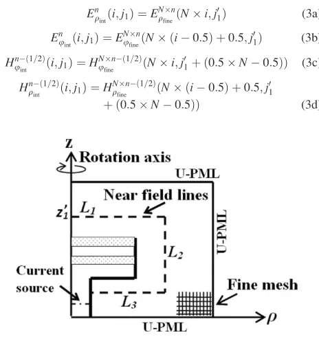
In this article, we introduce for the first time a new approach using the multiresolution technique known as the dual-grid (DG) method [12] to simulate electrically large BoR structures in cylin-drical coordinates system. The test example selected here is a par-abolic antenna system [Fig. 1(b)] illuminated by an electromag-netic band gap (EBG) resonator antenna [Fig. 1(a)] [13]. We show that the proposed numerical scheme leads to much shorter compu-tational time without scarifying the accuracy of the simulation. 2. DESCRIPTION OF THE DG SCHEME IN BoR-FDTD

The DG scheme consists in dividing the electromagnetic prob-lem into two successive simulation steps.

2.1. Step 1: Fine Analysis of the Feed Parts

In the first simulation, only the feed is considered [Fig. 1(a)]. It is discretized using a fine mesh for good structural approxima-tion. The computational volume is represented in Figure 2. It is limited by unsplit perfectly matched layers to simulate an infi-nite open problem. The field data generated along the near-field contours L1 to L3 are stored at each time step throughout the simulation. At the end of this simulation, the characteristics of the isolated feed are determined.

2.2. Step 2: Coarse Analysis of the Whole Antenna System

Once the first simulation is completed, the second one is launched [Fig. 1(b)]; a coarser FDTD mesh is selected to describe the whole antenna structure. The near-field data stored along the field lines in the first simulation are used as excitation sources in the second run. The ‘‘total field/scattered field’’ (TF/SF) decomposition is then applied to inject these fields into the coarse simulation domain [9]. As a consequence, the coarse simulation is divided into two field regions [Fig. 1(b)], both regions being separated by the excitation lines. The feed part is now totally encapsulated inside the scat-tered-field region and is thus considered as part of the scatterer.

2.3. Interpolation and Sampling in Space Domain

fields in Step 1. We have found that the use of linear interpola-tion is sufficient to guaranty smooth field variainterpola-tions.

For this purpose, it is important to note that, in any BoR-FDTD lattice, the first cell in q–direction is defined to be half the size of the adjacent cells [3, 9]. If Nis an arbitrary integer number defining the mesh size ratio between the first and second simulations, respectively

N¼Dqcoarse Dqfine

¼Dzcoarse Dzfine

(1)

then the mesh size ratio of the first cell inq-direction is equal to

N/2. IfNis an odd number, this value is not an integer whereas it remains an integer if Nis an even number. Therefore, depend-ing on the parity of N, the fields in the fine FDTD simulation must be properly identified to interpolate or sample the values for the coarse simulation. Because of this reason, separate sets of equations must be used to handle odd and even values ofN.

We outline below the scheme needed for the linear interpola-tion and sampling of the field components in space. We only consider one of the three contour lines, the other two lines being treated in a similar manner. We select here the contour line L1 (z¼const:¼z0₁, where z10 is the line path of L1 in z-direction in the fine FDTD mesh [Figs. 1(b) and 2].

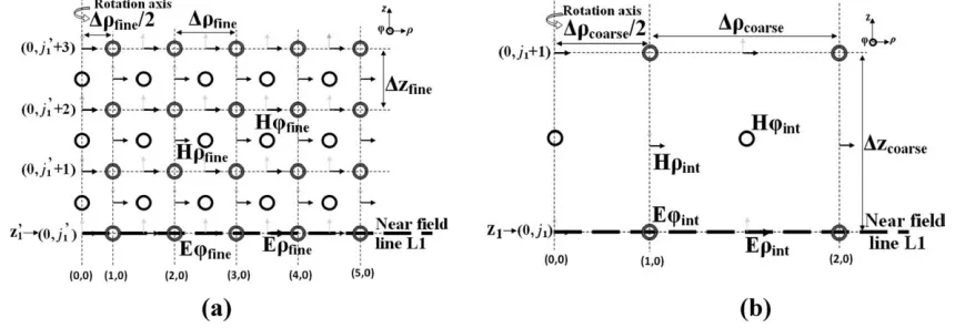
First, let us suppose thatN is an even integer. As an exam-ple, Figure 3 illustrates the field configurations for the fine and coarse meshes withN ¼2. A set of general space interpolation equations Eq. (2) for all even mesh ratios (N ¼ 2, 4, 6, etc.) along path L1 is derived (here, we assume that Dz ¼ Dq; but Eq. (2) remain the same if Dq =Dzbecause the mesh ratio is identical in both directions [Eq. (1)]

En_u

intði;j1Þ ¼ 1 2E

Nn

ufineðN ði0:5Þ þ1;j 0 1Þ

þ1 2E

Nn

ufineðN ði0:5Þ;j 0 1Þ

(2a)

En

qintði;j1Þ ¼E

Nn

qfineðNi;j 0

1Þ (2b) Hn_qð1=2Þ

int ði;j1Þ ¼ 1 4H

Nnð1=2Þ

qfine ðN ði0:5Þ þ1;j 0

1þ0:5NÞ þ1

4H Nnð1=2Þ

qfine ðN ði0:5Þ;j 0

1þ0:5NÞ þ1

4H

Nnð1=2Þ

qfine ðN ði0:5Þ þ1;j 0

1þ ð0:5N1ÞÞ þ1

4H

Nnð1=2Þ

qfine ðN ði0:5Þ;j 0

1þ ð0:5N1ÞÞ (2c)

H_unð1=2Þ int ði;j1Þ ¼

1 2H

Nnð1=2Þ

ufine ðNi;j 0

1þ0:5NÞ þ1

2H

Nnð1=2Þ

ufine ðNi;j 0

1þ ð0:5N1ÞÞ

(2d)

whereEintandHintare the interpolated field components, andEfine andHfinerefer to the field components of the fine FDTD mesh.j1 andj10are the coordinate indexes ofz1andz10for line pathL1in the coarse and fine meshes, respectively (z1¼Dzcoarsej1, z01¼Dzfinej01). In these equations,iis the cell index inq -direc-tion for the coarse FDTD domain (i¼1, 2, 3, …,imax). The value

imaxis given byimax¼imax fine=N, whereimax_fineis the maximum number of cells along pathL1 in the fine FDTD domain. As this value must be an integer,imax_finemust be able to be divided byN exactly. Note that the value ofEqint in Eq. (2b) is sampled from Eqfinein finer mesh (Fig. 3) because it lies at the same position. Other field values are calculated using linear interpolation.

Similarly, for odd values of N(N¼ 3, 5, 7, etc.), Figure 4 illustrates an example of field configuration for the fine and coarse grids assumingN¼3. Using the same notations, the gen-eral space sampling equations are given by

En_q

intði;j1Þ ¼E

Nn

qfineðNi;j 0

1Þ (3a) En_u

intði;j1Þ ¼E

Nn

ufineðN ði0:5Þ þ0:5;j 0

1Þ (3b) H_unð1=2Þ

int ði;j1Þ ¼H Nnð1=2Þ

ufine ðNi;j 0

1þ ð0:5N0:5ÞÞ (3c) H_qnð1=2Þ

int ði;j1Þ ¼H Nnð1=2Þ

qfine ðN ði0:5Þ þ0:5;j 0 1

þ ð0:5N0:5ÞÞ (3d) Figure 1 DG scheme and antenna system used to assess the performance of DG-BoR-FDTD. (a) Double-layer 1D-EBG feed, and first DG step (fine mesh). (b) Whole antenna system, and second DG step (coarser mesh).k¼30 mm,kg¼k0=pffiffiffiffier; F¼21k0andD¼60k0

Once determined, the field dataEintandHintare saved; they will be used later in the second simulation as correction terms to the TF/SF update equations [9].

2.4. Sampling in Time Domain

As the mesh size of the second simulation is larger than in the first one, the stored data must comply with the stability criterion. Hence, they must be also interpolated in time domain in accord-ance with the applied mesh ratio N. The linear time domain interpolation requires that the fields at time index nandn þ 1 of the first FDTD simulation to be weighted according to the time ratio between DtcoarseandDtfine. In all cases, we select the time step in the second FDTD simulation to be Dtcoarse ¼ N

Dtfine. As N is always assumed to be an integer number, this operation is thus equivalent to sampling in time domain. This consideration is incorporated in Eqs. (2) and (3). This ensures smooth continuity and stability of the fields.

3. NUMERICAL VALIDATIONS

To validate the proposed scheme, we selected a parabolic reflector antenna system as a benchmark case. In this example, we use one dimensional- (1D) EBG resonator antenna with double disk layers as shown in Figure 1 to illuminate the reflector [14]. The antenna is designed at 10 GHz (k0 ¼ 30 mm) and the relative dielectric permittivity of the EBG layers equals 10.2. The advantage of using a 1D-EBG antenna as a feed lies in its directive radiation pattern and its small overall size, reducing the shadowing effect for the overall system. The reflector is a parabolic dish with a diameter size of 60k0and a focal length to diameter ratio (F/D) of 0.35.

In terms of analysis, the feed must be discretized finely to describe accurately its features, whereas the reflector does not need such a fine mesh due to its large size and simple design.

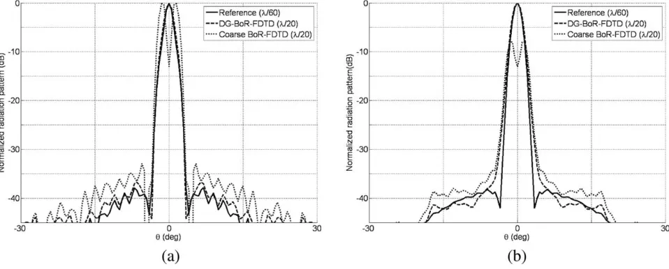
We first validate the feed antenna using the DG technique to show the advantage of using this approach over the classical BoR-FDTD. To this end, Figure 5 compares the radiation pat-terns computed using three approaches

1. Classical BoR-FDTD with a fine mesh (k0/60,Dq¼Dz¼

0.5 mm): the corresponding solution is the reference one. The FDTD mesh is fine enough to describe accurately all the features of the 1D-EBG antenna,

2. Classical BoR-FDTD with a coarser mesh (k0/20, Dq ¼

Dz¼1.5 mm),

3. DG-BoR-FDTD: in this case, the feed antenna is simulated as illustrated in Figure 2 with the fine mesh resolution (k0/ 60). The near-field distribution is saved after being interpo-lated with mesh ratio N¼ 3, and these data are reradiated in far field in free space using the coarse mesh (k0/20). This figure shows that the DG technique is in very good agreement with the reference solution whereas the simulation using solely coarser mesh is clearly inaccurate.

Next, we consider the entire parabolic antenna structure. We simulate it using the fine mesh simulation (k0/60, classical BoR-FDTD) and compare its radiation patterns with those generated with the classical coarse BoR-FDTD (k0/20) and the DG tech-nique. As the first DG step has been already performed (Fig. 5), the saved data can be reused for the second step; in this case, the parabolic reflector is described coarsely, as illustrated in Fig-ure 1(b). Note that the feed structFig-ure is retained in this simula-tion as part of the scatterer. The final results are represented in Figure 6 at 10 GHz. The agreement between the DG technique and the fine BoR-FDTD result is excellent. As expected, the classical coarse BoR-FDTD run shows inaccurate result. Figure 3 Configuration of the field components in the BoR-FDTD lattice. (a) Fine mesh. (b) Coarse mesh (two times coarser,N¼2)

Table 1 compares the main simulation features for classical fine and DG-BoR-FDTD. The latter have been launched on a 2-GHz Intel machine with 1 GB RAM. This Table shows that the total time needed to perform simulation using the DG technique is only 14 min, compared to 2.4 h using the classical fine BoR-FDTD approach. The execution time and memory resources are reduced by a factor 10 and 2.5, respectively, compared to the reference case.

4. CONCLUSIONS

The DG-BoR-FDTD technique has been introduced to analyze effectively large axis-symmetrical problems. The proposed

approach combines two successive BoR-FDTD simulations with different mesh resolutions. The implementation procedure has been described with emphasis on the mechanisms used to link both BoR-FDTD volumes, namely the linear interpolation or sampling in time and space domains, and the TF/SF decomposi-tion. The set of general equations has been derived depending on the parity of the mesh ratio value between the fine and coarse BoR-FDTD meshes in the DG scheme.

The proposed algorithms have been validated successfully by comparing the numerical results obtained with the fine classical BoR-FDTD and the DG-BoR-FDTD. Provided that the mesh ra-tioN is unchanged, the saved near-field data can be repeatedly used (second simulation of the DG algorithm) without repeating the expensive computational part of the calculation (first simula-tion of the DG technique). The DG scheme reduces simulasimula-tion time and memory considerably and paves the way for efficient full-wave optimizations in the future.

ACKNOWLEDGMENTS

This work was performed using HPC resources from GENCI-IDRIS (grant 2010-050779). The authors thank the ‘‘Universite Europeenne de Bretagne’’ and the ‘‘Conseil Regional de Bretagne’’ Figure 5 1D-EBG antenna. Copolarization component computed in far field at 10 GHz using classical fine BoR-FDTD (reference), DG-BoR-FDTD and classical coarse BoR-FDTD. (a) E-plane and (b) H-plane

Figure 6 Whole reflector antenna system. Copolarization component computed in far field at 10 GHz using classical fine BoR-FDTD (reference), DG-BoR-FDTD and classical coarse BoR-FDTD. (a) E-plane and (b) H-plane

TABLE 1 Parameters of the Simulations

Fine BoR-FDTD

DG-BoR-FDTD

Step 1 Step 2

Mesh sizeNqNz 1242969 92411 418330

Time steps 0.586 ps 0.586 ps 1.760 ps

Computation time 2.4 h 1 min 13 min

for their financial support (project acronyms: OPTIMISE, CRE-ATE/CONFOCAL, and GRAPPAS).

REFERENCES

1. http://www.ticra.com/. 2. http://www.mician.com.

3. Y. Chen, R. Mittra, and P. Harms, Finite-difference time-domain algorithm for solving Maxwell’s equations in rotationally symmet-ric geometries, IEEE Trans Microwave Theory Tech 44 (1996), 832–839.

4. A. Rolland, M. Ettore, M. Drissi, L. Le Coq, and R. Sauleau, Opti-mization of reduced-size smooth-walled conical horns using BoR-FDTD and genetic algorithm, IEEE Trans Antennas Propag 58 (2010), 3094–3100.

5. M. Celuch and W.K. Gwarek, Industrial design of axisymmetrical devices using a customized solver from RF to optical frequency bands, IEEE Microwave Mag 9 (2008), 150–159.

6. A. Rolland, M. Ettore, A.V. Boriskin, L. Le Coq, and R. Sauleau, Axisymmetric resonant lens antenna with improved directivity in Ka-band, IEEE Antennas Wireless Propag Lett 10 (2011), 37–40. 7. Z. Yang, Y. Chen, W. Yu, and R. Mittra, Hybrid FDTD/AutoCAD

method for the analysis of BoR horns and reflectors, Microwave Opt Technol Lett 37 (2003), 236–243.

8. M.S. Tong, R. Sauleau, A. Rolland, and T.G. Chang, Analysis of electromagnetic band-gap waveguide structures using body-of-revo-lution finite-difference time-domain method, Microwave Opt Tech-nol Lett 49 (2007), 2201–2206.

9. A. Taflove and S.C. Hagness, Computational electrodynamics: The finite-difference time-domain method, 2nd ed., Artech House, Nor-wood, MA, 2000.

10. C. Bruns, P. Leuchtmann, and R. Vahldieck, Comprehensive analy-sis and simulation of a 1-18 GHz broadband parabolic reflector horn antenna system, IEEE Trans Antennas Propag 51 (2003), 1418–1423.

11. M. Arrebola, L. Haro, and J. Encinar, Analysis of dual-reflector antennas with a reflectarray as subreflector, IEEE Antennas Propag Mag 50 (2008), 1418–1423.

12. R. Pascaud, R. Gillard, R. Loison, J. Wiart, and M.F. Wang, Dual-grid FDTD scheme for fast simulation of surrounded antenna, IET Microwave Antenna Propag 3 (2007), 700–706.

13. R. Chantalat, C. Menudier, M. Thevenot, T. Monediere, E. Arnaud, and P. Dumon, Enhanced EBG resonator antenna as feed of a reflector antenna in the Ka-band, IEEE Antennas Wireless Propag Lett 7 (2008), 349–352.

14. A.A. Kishk, One-dimensional electromagnetic bandgap for directiv-ity enhancement of waveguide antennas, Microwave Opt Technol Lett 47 (2005), 430–434.

VC_{2012 Wiley Periodicals, Inc.}

INTEGRATION OF MONOPOLE SLOT AND

MONOPOLE STRIP FOR INTERNAL

WWAN HANDSET ANTENNA

Kin-Lu Wong and Po-Wei Lin

Department of Electrical Engineering, National Sun Yat-Sen University, Kaohsiung 804, Taiwan; Corresponding author: [email protected]

Received 13 September 2011

ABSTRACT:A novel internal handset antenna formed by a monopole slot and a monopole strip for the wireless wide area network (WWAN) operation in the 824–960 and 1710–2170 MHz bands is presented. The monopole strip is disposed in the monopole slot, and both are embedded in the system ground plane of the handset with a small board space of 9

40 mm2at about the bottom edge of the circuit board. The monopole strip serves as a feed for the monopole slot and also functions as an

efficient radiator. In the proposed design, the monopole slot generates a quarter-wavelength slot mode in the antenna’s lower band, while the monopole strip contributes its quarter-wavelength mode in the antenna’s upper band. By including a vertical strip that can be enclosed inside the handset casing or be a part of the bezel surrounding, the periphery of the handset casing and connected to the bottom edge of the system ground plane, the impedance matching of the excited slot mode can be greatly improved. In this case, the proposed antenna can provide two wide operating bands with good impedance matching to cover the pentaband WWAN operation. Detailed operating principle of the integrated monopole slot and monopole strip for the internal WWAN handset antenna is described. The proposed antenna is also fabricated and obtained results are presented and discussed.VC _{2012 Wiley Periodicals,} Inc. Microwave Opt Technol Lett 54:1718–1723, 2012; View this article online at wileyonlinelibrary.com. DOI 10.1002/mop.26870

Key words:mobile antennas; handset antennas; monopole slot antennas; monopole; strip antennas; wireless wide area network antennas

1. INTRODUCTION

The monopole slot is easy to fabricate and can operate at its quarter-wavelength mode as the lowest resonant mode [1–3], which makes it promising to achieve wideband operation with a small size for mobile handset applications. Recently, several printed monopole slot antennas covering the wireless wide area network (WWAN) operation in the mobile handset have been demonstrated [4–12]. These reported monopole slot handset antennas for the WWAN operation are mainly excited using a microstrip feedline, which is generally not an efficient radiator for frequencies in the desired operating bands of the antenna. As the monopole slot is a no-ground or clearance region embedded in the system circuit board of the handset, it is expected that a monopole strip disposed inside the monopole slot can be an effi-cient radiator and may contribute resonant modes in the desired operating bands of the antenna, if properly designed. In this case, the monopole strip not only can serve as a feed for the monopole slot but also can function like an efficient radiator to generate additional resonant modes in the antenna’s desired operating bands. This can result in much wider operating bands achieved for the antenna. This design concept is implemented in this study.