Mathematical and Numerical Modeling of the Coupled Dynamic Thermoplastic Problem

(1)

Mathematical and Numerical Modeling of the

Coupled Dynamic Thermoplastic Problem

Yusupov Y.1,*_{, Khaldjigitov А.А.}2

1_{Faculty of Mathematics, National University of Uzbekistan, Uzbekistan} 2_{Samarkand Branch of Tashkent University of Information technologies, Uzbekistan}

Abstract

Using the strain space and deformation thermoplasticity theories the coupled dynamic thermoplastic boundary value problems are formulated. Strain space thermoplasticity theory, in contrast to the deformation one, allows formulating the coupled thermoplastic boundary value problems for the displacement and temperature increments. As an example, in one-dimensional case, the explicit and implicit types of finite difference equations are constructed. The numerical solution of the explicit finite difference equations reduced to the application of the recurrent formulas, whereas the implicit scheme reduced to the application of the elimination method. Comparison shows that the numerical results obtained using explicit and implicit scheme coincides.

Keywords

Finite Difference, Elimination Method, Coupled, Thermoplastic, Dynamic, Strain Space Theory, Deformation Theory, Displacement, Temperature, Explicit, Implicit

1. Introduction

Thermo-mechanical coupling is the most common class of coupled problems, in which the mechanical response of the structure depends on its thermal behavior and vice versa. Investigations the in the field of coupled thermoelasticity and thermoplasticity are enormously developed due to their many applications in the advanced structural design problems.

In case of coupled thermoelasticity and thermoplasticity boundary value problems, the motion equation, constitutive relations are considered in conjunction with the heat conduction equation. It should be noted, that the temperature and its derivative are included in the motion equation, and the heat equation contains a strain tensor. The heat conduction equation, under certain conditions, can be

considered and solved separately from the motion equations. Coupled thermoelasticity problems investigated by Biot [1], Lord & Shulman [2], Yousuf [3], where has been introduced a generalized coupled theory with a wave-type heat equation. The coupled thermoplasticity problems for anisotropic materials at finite deformations are considered in [10].The thermoplasticity coupling problems are considered in Slodrbach [4], Canadjia and Brnik [5]. The coupled visco-plasticity is considered by Stainier and Ortiz [9]. In [6] the coupled thermoplasticity problem is formulated using the strain space plasticity theory, which has advantages comparison to stress space [19] one. Thermomechanical coupled and uncoupled boundary value problems are solved in following works [7, 8, 11, 12, 13, 14].

This paper deals with the numerical solution of the coupled thermoplastic boundary value problems formulated using the deformation thermoplasticity theory [16] and strain space thermoplasticity [7]. Coupled thermoplasticity boundary problem based on deformation theory may be solved as a thermoelasticity problem i.e. is not required the partition of the problem. Usually in numerical solution of strain space thermoplasticity problems the original problem is partitioned into several smaller sub-problems, which are solved sequentially. Note that, strain space coupled thermoplasticity problem in difference from the stress space one is not depend on stress tensor.

(2)

2. Formulation of the Coupled

Thermoplasticity Boundary Value

Problems

Coupled thermoplasticity problems depending on which theory of thermoplasticity deformation or flow theory is used, can be formulated two types of coupled thermomechanical boundary value problems. Usually the coupled thermoplasticity boundary value problems consist of motion equation, constitutive relations and heat equations with a corresponding initial and boundary conditions. Usually in numerical solution of coupled thermoplasticity problems the original problem is partitioned into several smaller sub-problems, which are solved sequentially. In case of coupled thermoplasticity boundary problems, based on deformation theory, is not required the partition of the problem. Coupled thermoplasticity boundary value problems may be formulated using the stress space and strain space flow theories. Note that the strain space thermoplasticity theory [7] in comparison with stress space one [19] more suitable for the formulating and numerical solution of the coupled boundary value problems.

2.1. The Coupled Boundary Value Problem Using Deformation Theory of Thermoplasticity

The coupled thermoplastic boundary value problem using deformation theory consists of the motion equations

, ,

ij j Xi ui

σ + =ρ (1) Constitutive relation of the deformation theory [16]

( 3 ) u ,

ij ij ij

u

K σ e

σ θ αϑ δ

ε

= − + ₍₂₎

heat conduction equation [15]

0 ,Tii C T Tε 0 (3 2 ) ij 0 λ − − ⋅α λ+ µ ε⋅  = (3) and Cauchy relations

(

, ,

)

1 2

ij ui j uj i

ε = + (4)

with the corresponding initial

0 , 0 , 0 0

it t i i t t i t t

u ₌ =φ u ₌ =ψ T ₌ =T ₍₅₎ and boundary conditions

1 1 2

0 0

0

, , ,

i i ij j i

u _∑ u T _∑ T

σ

n S

∑

= = = ₍₆₎

where Cε − heat at a constant temperature,

α

−

thermal

expansion coefficient,

λ

₀

−

the heat flow coefficient,

−

µ

λ

,

Lame constants

,

θ

−

spherical part of strain tensor, 0

T T

ϑ = −

-

temperature difference, X_i−volume force, −

ρ density of the body, δij − kronecker symbol,

2 3

K = −λ µ

,

In Eq.(2) the value

σ

_u

,

in case of a piecewise linear deformation diagram may be replaced by the expression

*

2 2( )( )

u u u u

σ = µε − µ µ ε− ′ −ε

where µ′ − tangent modulus,

σ ε

_u

,

_u- intensity of stress and strain tensors. Taking into account the last relation the eq. (1 - 6) in one dimensional case take the form

2 11

1 2

u X

x t

σ _ρ

∂ ∂

+ =

∂ ∂ (7)

* 11 ( 2 ) 11 ( 0) 4₃( )(1 u) 11

u

T T ε

σ λ µ ε αγ µ µ ε

ε ′

= + − − − − − ₍₈₎

11 u_x

ε =∂

∂ (9)

Substituting the Eq. (8) and Eq. (9) into Eq. (7) gives the motion equation in terms of displacements

2 2 2

0

2 2 2

4

( 2 ) ( ) ( )

3

u _{T T} u u

x x t

λ+ µ ∂ −αγ − − µ µ− ′ ∂ =ρ∂

∂ ∂ ∂ (10)

where γ =3λ+2µ

The heat equation in one dimensional case has the form

2 2

0 2 0 0

T _C T _T u t x t x ε

λ ∂ − ∂ −αγ ∂ =

∂ ∂ ∂

∂ (11)

with the appropriate initial and boundary conditions

( )

0

0 0

, ( ),

( ), ,

i t

t

u x t x u _x t

T x t T

φ

ψ =

=

 =

 ∂ ₌  ∂ 

 ₌



(12)

( )

0 0

0

1 2

0

, , , ,

x x

u x t u u x t u T x t T t T x t T t

= =

 = =

 

= =





(13)

where



−

the rod length. eq. (10-13) present the coupled boundary value problem for deformation theory of thermoplasticity in one dimensional case.

2.2. The Coupled Thermoplasticity Boundary Problem Using the Flow Theory

The coupled boundary problem based on the strain space thermoplasticity theory consists of motion equation written for increments of unknown quantities

,

ij j i i

dσ +dX =ρdu₍₁₄₎

(3)

(

)

2

,

2 2

0 0;

d _ij d _ij d _ij dT _ij

F e de_kl _kl e_ij e_{ij T} dT

u u

F

F and dF e de_ij _ij dT

T

σ λ θδ µ ε αγ δ

µ µ µ µ

∂ ε ε ∂ = + − − ′ ′ − − ∂ − − ∂ = = + ≥ (15)

differentiated heat conduction equation for isotropic materials [15]

0dT,ii C dT Tε 0 d ij 0

λ − − αγ ε = ₍₁₆₎

and differentiated Cauchy relations

(

, ,

)

1

2

ij i j j i

dε = du +du ₍₁₇₎

with initial

0 0

, ,

it t i i t t i

t t

d u du

dT T φ ψ = = =  = =   ₌  (18)

and boundary conditions

1 1 2 0 0 0 , , i i

ij j i

du u dT T d nσ S

∑ ∑ ∑  = =   =

 (19)

where

e

_ij

−

deviator of the strain tensor, T −

temperature, Cε − heat at a constant temperature,

α

−

thermal expansion coefficient,

λ −

0 the heat flow coefficient and

F

−

loading function in the strain space [7]

(

)

1 _, ₀

2 ij ij

F ≡ e e −R ω T = (20)

Eq. (14-19) in one dimensional case for piecewise line of deformation diagrams take following form

2 11

1 2

(d ) _dX ( )du

x t

σ _ρ

∂ ₊ ₌ ∂

∂ ∂ (21)

11 11

( 2 )

4₍ ₎ 3( )

3

d d dT

F

d dT

T

σ λ µ ε αγ

µ µ µ µ ε

ε = + − − ′ − ∂ ′ − − − ∂ (22)

11 ( )du

d

x

ε =∂

∂ (23)

Substituting Eq. (23) into Eq. (22) gives

11 ( 2 ) ( )

4₍ ₎ ( ) 3( ) 3

du

d dT

x

du _{F dT}

u

x T

x

σ λ µ αγ

µ µ µ µ ∂ = + − − ∂ ′ ∂ − ∂ ′ − − − _∂ ∂ ∂ ∂ (24)

and then inserting into Eq. (21) gives motion equation for differentials of displacements and temperature

2 2 2 2 2 2 2

4 ( ) ( )

( 2 ( ))

3 ( ) ( ) 3( ) ( ) du dT x x

dT u _dT u

du

x x x

u t

x

λ µ µ µ αγ

µ µ β ρ

∂ ∂ ′ + − − − − ∂ ∂ ∂ ∂ ₋ ∂ ∂ ∂ ∂ ∂ ′ − − _∂ = ∂ ∂ (25)

where β = ∂F T∂ . The following heat equation together with a Eq. (25)

2 2

0 2 0

(dT) _C (dT) _T (du) ₀

x ε t x t

λ ∂ − ∂ − αγ ∂ =

∂ ∂ ∂ ∂ (26)

with an appropriate initial and boundary conditions

( )

0 0 0 0 , ( ), ( ) _{( ),} , i t i t t

d u x t x du _x

t

dT x t T

φ ψ = = =  =  ∂ ₌  ∂   ₌  (27)

( )

0 0 0 1 0 2 , , , , , , , x x x x

du x t u du x t u

d T x t T t

= = = =  = =  ₌   =    (28)

presents the 1D coupled thermoplasticity boundary value problem for strain space theory. Where

0

, , , , , ,Cε

λ µ µ α β′ λ − are the given values,



−

the rod length, φ ψ, ,T T T₀, ,₁ ₂− are the known values.

3. Explicit and Implicit Finite Difference

Equations

For the formulated in the preceding paragraphs coupled thermoplasticity boundary problems using the finite difference method an explicit and implicit schemes are constructed. Note that, in case of strain space thermoplasticity theory the discrete equations are written for displacement and temperature increments. The explicit schemes consist of two recurrent formulas displacement u

and temperature T increments, whereas the implicit schemes take the suitable form for the application the elimination method [18]. Note that in the case of strain space thermoplasticity theory the external thermomechanical forces are gradually applied with a small increments and the results are found as a sum of the increments of corresponding values.

3.1. Finite Difference Equations for 1D Coupled Boundary Problem on Deformation Theory of Thermoplasticity

(4)

1 1

1 1 1 1

2 2

4

( 2 ( ))

3 2

j j j j j j j j

i i i i i i i i

u u u T T u u u

h h

λ µ µ µ αγ ρ

τ

+ −

+ − + − + − − − +

′

+ − − − = (29)

1 1 1 1 1 1

0 2 0

2 ₀

2 4

j j j j j j j j j

i i i i i i i i i

T T T _C T T _T u u u u

h ε h

λ αγ

τ τ

+ − + + − −

+ − + − ₊ − ₋ + − − − + + − ₌ ₍₃₀₎

Solving the finite difference Eq. (29) and Eq. (30) for j 1

i

u + _and j 1

i

T + _{respectively, we get}

1 1 1 1

2 2

1 1

2

2 ( 2 )

2 ₂

2 4 ( ) 3

j j j j j

i i i i i

j j j

i _j _j _j i i

i i i

u u u T T

h h

u u u

h

λ µ αγ

τ ρ µ µ + − + − + − + −  ₊ − + ₋ − ₋     = + −  _′ − +  − −     (31)

1 1 1 1

1 1 1 1 1 1 1 1

0 2

2 2

4

j j j j j j j

j i i i j i i i i j

i T T T i u u u u i

T T T

Cε h h

τ λ αγ

τ

+ + − −

+ ₌  + − + − ₋ + − − − + + − ₋ −

 

  (32)

Eq. (31) and Eq. (32) allow us to find the values of u x t( , ) and T x t( , ) at the layer

t

j+1 using the given values of these functions at the two previous layers. The values of u x t( , )on two primary layers j=0 and j =1 can be found from the initial conditions, and the values of T x t( , ) can be obtained from the following finite difference relations

0 0 0 0 0

1 1 1 1

2 2

1 0

0 0 0

1 1

2

2 ( 2 )

1 2 ₂ ₂

2 _{4 (} ₎ 2

3

i i i i i

i i

i i i

u u u T T

h h

u u

u u u

h

λ µ αγ

τ _ψτ ρ µ µ + − + − + −   ₊ − + ₋ − ₋          = + +   ₋ ₋ _′ − +      _ _    (33)

1 1 0 0 0 0 0

1 1 1 1 1 1 1 0

0 0 2

2 2

2

i i i i i i i

i i

u u u u T T T

T T T

Cε h h

τ αγ λ

τ

+ − + − + −

 − − + − + 

= − _ − _−

  (34)

In the first term of the finite difference Eq. (29), replacing j into j+1, the equation can be reduced to the form

1 1 1

1 1

j j j

i i i i i i ij

a u + b u + c u + f

+ + + − = (35)

where

2 4

2 ( )

3 _,

i

a

h

λ+ µ− µ µ′−

= ₂ ₂

4

2( 2 ( ))

3 _,

i

b

h

λ µ µ µ _ρ

τ ′

+ − −

= − − 2

4

2 ( )

3

i

c

h

λ+ µ− µ µ− ′ =

1

1 1

2

2 (3 2 )

2

j j j j

i i i i

ij T T u u

f

h

α λ µ ρ

τ −

+ − − −

= + +

Similarly, we can write the finite difference Eq. (30) in the form

1 1 1

1 1

j j j

i i i i i i ij

a T + b T + c T + f

+ + + − = (36)

where 0 2

,

i

a

h

λ

=

0 2 2 2 _, i b h λ ρ τ

= − − 0

2, i c h λ =

1 1 1 1 1

1 1 1 1

4 2

j j j j j

j i i i i i

ij i u u u u T

f T C

h ε β τ τ + + − − − + − − − + + − = −

(5)

3.2. Finite Difference Equations for 1D Coupled Strain Space Thermoplasticity Problem Substituting the finite difference quotients into Eq. (25-26) give

1 1 1 1

2

1 1 1 1 1 1 ₁ ₁

2 2 2 1 1 2 4

( 2 ( ))

3 2 2 2 2 2 3( ) ( ) 2

j j j j j

i i i i i

j j j j j j j

j

i i i i i i i _j _j _j

i

i i i

j j

i i

du du du dT dT

h h

dT dT u u _dT u u u

du du du

h h h

u u

h

λ µ µ µ αγ

µ µ β ρ

τ + − + − + − + − + − + − + − − + − ′ + − − − − − − ₋ − + − + ′ − − = − (37)

1 1 1 1 1 1

0 2 0

2 ₀

2 4

j j j j j j j j j

i i i i i i i i i

dT dT dT _C dT dT _T du du du du

h ε h

λ αγ

τ τ

+ − + + − −

+ − + − ₊ − ₋ + − − − + + − ₌ ₍₃₈₎

Solving the discrete Eq. (37-38) for the j 1

i

du + _and j 1

i

dT + _{we can find the following explicit recurrent formulas}

1 1

2

1 1

2 ₂

1 1 1

2 1 1

1 1 1 1

2 1 1

2 4

( 2 ( )) 3

2

2 ₍ ₎

2

2 2

3( )

( )

2

j j j

i i i

j j j

j i i i

j j _i

j i i j

i j j i

i i

j j j j

i i i i

j j

i i

du du du

h

u u u

dT

dT dT _h

du du

u u

h

dT dT u u

h h

u u

h

λ µ µ µ

τ _αγ ρ

µ µ β

+ − + − + + − + − + − + − + −       − +  ₊ ₋ ₋ _′ ₋     − +   −   = _− − − +_ − −      ₋ ₋    − − ′ ⋅  −       1 j i du − (39)

1 1 1 1

1 1 1 1 1 1 1 1

0 2

2 2

4

j j j j j j j

j j i i i i i i i j

i i du du du du dT dT dT i

dT T dT

Cε h h

τ αγ λ

τ

+ + − −

+ _{= −}  + − − − + + − ₋ + − + − ₋ −

 

  (40)

Eq. (39-40) allows to find the value of du x t( , ) and dT x t( , ) using the known values at the preceding two layers. The values of du x t( , ) and dT x t( , ) on the initial two j =0and j =1 may be find using the initial and

boundary conditions

0 0 0 0 0

1 1 1 1

2 2

1 0

0 0 0

1 1

2

2 ( 2 )

1 2 ₂ ₂

2 _{4 (} ₎ 2

3

i i i i i

i i

i i i

du du du dT dT

h h

du du

du du du

h

λ µ αγ

τ _ψτ ρ µ µ + − + − + −   ₊ − + ₋ − ₋          = + +   _′ − +   − −    _ _    (41)

1 1 0 0 0 0 0

1 1 1 1 1 1 1 0

0 0 2

2 2

2

i i i i i i i

i du du du du dT dT dT i

dT T dT

Cε h h

τ αγ λ

τ

+ − + − + −

 − − + − + 

= − _ − _−

  (42)

Replacing index j by j+1 for the first term of the Eq. (37) the finite difference equation can be rewritten in the following form

1 1 1

1 1

j j j

i i i i i i ij

a du

+

b du

+

c du

+

f

+

−

=

(43)

where

2

4

2 ( )

3 _,

i

a

h

λ+ µ− µ µ′−

= ₂ ₂

4

2( 2 ( ))

3 _,

i

b

h

λ µ µ µ _ρ

τ

′

+ − −

= − − ₂

4

2 ( )

3

i

c

h

(6)

1 1 1 1

1 ₂

1 1

2

1 1 1 1

2

2 ₂

(3 2 ) 3( ) ( )

2 ₍ ₎

2 2

j j j j j

j

i i i i i

j j j j _i

i i i i

ij j j j j

i i i i

dT dT _dT u u u

dT dT du du _h _h

f

u u u u

h

h h

α λ µ ρ µ µ β

τ

+ − + −

−

+ −

+ − + −

− − +

− − _′

= + + + − −

− −

By analogy, the Eq. (38) takes the form

1 1 1

1 1

j j j

i i i i i i ij

a dT + b dT + c dT + f

+ + + − = (44)

where

0 2,

i

a h

λ

= 0

2

2 ,

2

i C

b

h ε

λ τ

= − − 0

2

i

c h

λ

=

1 1 1 1 1

1 1 1 1

4 2

j j j j j

j i i i i i

ij i du du du du dT

f T C

h ε

β

τ τ

+ + − − −

+ − − − + + −

= −

For solving the Eq. (43-44), the elimination method [18] is applied, and the resulting displacement and temperature are found as a sum of increments of du x t( , ) and dT x t( , ) i.e.

, p

u=

∑

du

p T=

∑

dT

where p – number of increments.

4. Numerical Tests

Let us consider the rod with the length



and inter

T

₀and boundary

T

₁

,

T

₂ temperatures on the both fixed sides, respectively. At the initial moment t=0_{along to the rod is applied a sinusoidal load. The described process using the} deformation of thermoplasticity can be modeled by the Eq. (10–13) with a following initial and boundary conditions:

( )

0

( )

0 0

0

( , )

, _t sin , 0, , _t ,

t

x u x t

u x t T x t T

t

π

= =

= ∂

 

= _ _ = =

∂   

( )

, _x ₀ 0,

( )

, _x ₁ 0,

( )

, _x ₀ 1,

( )

, _x ₁ 2

u x t ₌ = u x t ₌ = T x t ₌ =T T x t ₌ =T ,

The values of the constants were chosen as follows: 1.2

λ= _,λ0 =0.8, α =0.01, µ=0.5, ρ=1.0, Cε =3.5, n=15, τ=0.01, =1,

0 90

T = _,T₁=80_,T₂ =100_.

In case of the strain space thermoplasticity theory the considered rod problem may be described by the Eq. (25-28). Note, in case of strain space thermoplasticity theory the original problem is partitioned into several smaller sub-problems, which are solved sequentially. Therefore, Eq. (25-28) are obtained depending on the differentials (increments) of the temperature and displacement.

Discrete equations for coupled boundary value problems formulated on the basis of two thermoplastic theories were constructed using the finite difference method. In the previous section, the explicit and implicit finite difference schemes have been drawn up for each task. The explicit schemes are solved using the recurrent formulas for displacement u and temperature T. For solving the implicit schemes are applied the elimination method [18]. For the numerical solution of the finite difference equations was developed software in language C # integrated with Mathcad [20].

(7)

[image:7.595.64.547.91.617.2]

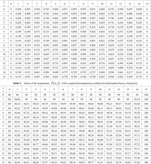
Table 1. Values of the displacement u x t( , ) of the coupled thermoplasticity problem for deformation theory of plasticity x

t 0 1 2 3 4 5 6 7 8 9 10 11 12 13 14 15

0 0 0,208 0,407 0,588 0,743 0,866 0,951 0,995 0,995 0,951 0,866 0,743 0,588 0,407 0,208 0 1 0 0,208 0,406 0,587 0,742 0,865 0,950 0,993 0,993 0,950 0,865 0,742 0,587 0,406 0,208 0 2 0 0,206 0,405 0,585 0,740 0,862 0,947 0,990 0,990 0,947 0,862 0,740 0,585 0,405 0,206 0 3 0 0,205 0,402 0,582 0,736 0,858 0,942 0,985 0,985 0,942 0,858 0,736 0,582 0,402 0,205 0 4 0 0,202 0,399 0,577 0,730 0,851 0,935 0,977 0,977 0,935 0,851 0,730 0,578 0,399 0,203 0 5 0 0,199 0,394 0,571 0,723 0,843 0,926 0,968 0,968 0,926 0,843 0,723 0,572 0,395 0,200 0 6 0 0,196 0,388 0,564 0,714 0,833 0,914 0,956 0,956 0,914 0,833 0,714 0,565 0,389 0,197 0 7 0 0,192 0,382 0,555 0,704 0,821 0,901 0,943 0,943 0,901 0,821 0,704 0,557 0,383 0,193 0 8 0 0,188 0,374 0,545 0,692 0,807 0,886 0,927 0,927 0,886 0,807 0,692 0,547 0,376 0,190 0 9 0 0,184 0,366 0,534 0,678 0,791 0,869 0,909 0,909 0,869 0,791 0,678 0,536 0,368 0,186 0 10 0 0,179 0,357 0,522 0,663 0,774 0,851 0,890 0,890 0,851 0,774 0,663 0,524 0,360 0,181 0 11 0 0,174 0,347 0,508 0,647 0,755 0,830 0,868 0,868 0,830 0,755 0,647 0,510 0,350 0,177 0 12 0 0,169 0,336 0,493 0,629 0,735 0,807 0,845 0,845 0,807 0,735 0,629 0,495 0,340 0,172 0 13 0 0,164 0,325 0,477 0,609 0,712 0,783 0,819 0,819 0,783 0,712 0,609 0,480 0,329 0,166 0 14 0 0,158 0,313 0,461 0,588 0,688 0,757 0,792 0,792 0,757 0,688 0,588 0,461 0,317 0,161 0 15 0 0,152 0,301 0,443 0,566 0,663 0,730 0,764 0,764 0,730 0,663 0,566 0,443 0,305 0,155 0

Table 2. Values of the temperature T x t( , ) of the coupled thermoplasticity problem for deformation theory of plasticity x

t 0 1 2 3 4 5 6 7 8 9 10 11 12 13 14 15

0 80 90 90 90 90 90 90 90 90 90 90 90 90 90 90 100

1 80 84,86 90 90 90 90 90 90 90 90 90 90 90 90 95,14 100

[image:7.595.65.546.355.623.2]

(8)

[image:8.595.91.519.78.243.2]

Figure 1. The distribution of the displacement u x t( , ) based on the Table 3.

In solving the 1D coupled boundary problem formulated using strain space thermoplasticity theory the initial and boundary conditions should be divided by the number of increments p:

( )

₀

( )

₀ 0

0

( ( , ))

, _t sin / , 0, , _t / ,

t

x du x t

du x t p dT x t T p

t

π

= =

= ∂

 

= _ _ = =

∂   

( )

, _x ₀ 0,

( )

, _x ₁ 0,

( )

, _x ₀ 1/ ,

( )

, _x ₁ 2/

du x t ₌ = d u x t ₌ = dT x t ₌ =T p dT x t ₌ =T p

5

p= .

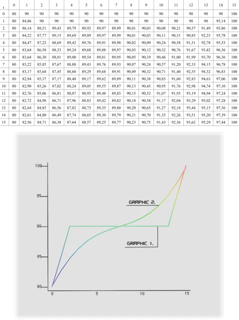
The numerical results for the coupled 1D strain space thermoplastic problem are given in the Tables 3-4. The result is obtained in solving the implicit schemes using elimination method. At the Fig.2 is shown the comparison of the initial (T0=90, T1=80, T2=100: GRAPHIC 1.) and calculated (GRAPHIC 2.) temperature distributions depending on time.

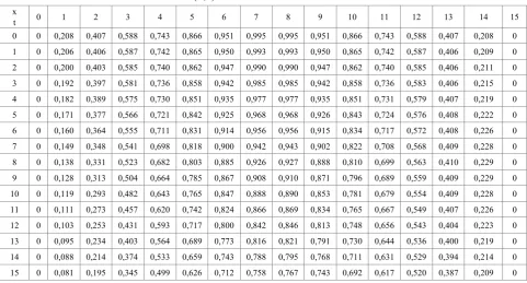
Table 3. Values of the displacement u x t( , ) of the coupled boundary problem for strain space thermoplasticity theory x

t 0 1 2 3 4 5 6 7 8 9 10 11 12 13 14 15

[image:8.595.64.546.431.690.2]

(9)

[image:9.595.62.545.88.693.2]

Table 4. Values of the temperature T x t( , ) of the coupled boundary problem for strain space thermoplasticity theory

t 0 1 2 3 4 5 6 7 8 9 10 11 12 13 14 15

0 80 90 90 90 90 90 90 90 90 90 90 90 90 90 90 100

1 80 84,86 90 90 90 90 90 90 90 90 90 90 90 90 95,14 100

2 80 86,14 88,51 89,43 89,79 89,92 89,97 89,99 90,01 90,03 90,08 90,21 90,57 91,49 93,86 100 3 80 84,22 87,77 89,15 89,69 89,89 89,97 89,99 90,01 90,03 90,11 90,31 90,85 92,23 95,78 100 4 80 84,47 87,22 88,69 89,42 89,76 89,91 89,98 90,02 90,09 90,24 90,58 91,31 92,78 95,53 100 5 80 83,64 86,58 88,33 89,24 89,68 89,88 89,97 90,03 90,12 90,32 90,76 91,67 93,42 96,36 100 6 80 83,64 86,30 88,01 89,00 89,54 89,81 89,95 90,05 90,19 90,46 91,00 91,99 93,70 96,36 100 7 80 83,22 85,85 87,67 88,80 89,43 89,76 89,93 90,07 90,24 90,57 91,20 92,33 94,15 96,78 100 8 80 83,17 85,68 87,45 88,60 89,29 89,68 89,91 90,09 90,32 90,71 91,40 92,55 94,32 96,83 100 9 80 82,94 85,37 87,17 88,40 89,17 89,62 89,89 90,11 90,38 90,83 91,60 92,83 94,63 97,06 100 10 80 82,90 85,26 87,02 88,24 89,05 89,55 89,87 90,13 90,45 90,95 91,76 92,98 94,74 97,10 100 11 80 82,76 85,06 86,81 88,07 88,93 89,48 89,85 90,15 90,52 91,07 91,93 93,19 94,94 97,24 100 12 80 82,72 84,98 86,71 87,96 88,83 89,42 89,82 90,18 90,58 91,17 92,04 93,29 95,02 97,28 100 13 80 82,64 84,85 86,56 87,82 88,73 89,35 89,80 90,20 90,65 91,27 92,18 93,44 95,15 97,36 100 14 80 82,61 84,80 86,49 87,74 88,65 89,30 89,79 90,21 90,70 91,35 92,26 93,51 95,20 97,39 100 15 80 82,56 84,71 86,38 87,64 88,57 89,25 89,77 90,23 90,75 91,43 92,36 93,62 95,29 97,44 100

[image:9.595.67.544.95.734.2]

(10)

The numerical results of the 1D coupled boundary value problems formulated using the deformation (Tables 1-2) and strain space (Tables 3-4) thermoplasticity theories show a good coincidence and thus establish the validity of the used modeling equations for describing the coupled thermoplasticity processes.

4. Conclusions

Using the strain space and deformation thermoplasticity theories two types of coupled boundary value problems are formulated. The coupled strain space thermoplastic boundary value problem more adequate describes the deformation process of the solids. In case of the strain space thermoplasticity problems the original problem is partitioned into several smaller sub-problems and the total deformation is composed from the strain increments corresponding to the increments of the external loads. Coupled thermoplasticity boundary problem based on deformation theory may be solved as a thermoelasticity problem i.e. is not required the partition of the problem. The explicit and implicit finite difference schemes are constructed and solved using the elimination method and recurrent formulas for displacement

u

and temperature T. For the numerical solution of the finite difference equations was developed software in language C # integrated with Mathcad [20].

Comparison of the numerical results received from the solving of the two types of 1D coupled thermoplasticity boundary value problems shows a good coincidence.

REFERENCES

[1] Biot, M.A. Thermoelasticity and irreversible thermo-dynamics. J. Appl. Phys., 1956, 27, 240–253. [2] Lord H.W., Shulman Y. A generalized dynamical theory of

thermoplasticity. J. Mech. Phys. Solids, 1967, vol.15, 299-309

[3] Youssef, H.M. Theory of two-temperature-generalized thermoelasticity. IMA J. Appl. Math., 2006, 71, 383-390 [4] Sloderbach, Z. Generalized coupled thermoplasticity taking

into account large strains: Part I. Conditions of uniqueness of the solution of boundary-value problem and bifurcation criteria. Math. and Mech of solids.2010, 15, 308-327. [5] Canadija M., Brnik J. Associative coupled thermoplasticity at

finite strain with temperature-dependent material parameters.

Int. J. Plasticity. 2004, 20, 1851-1874

[6] Khaldjigitov A.A, QalandarovA.A., Yusupov Y.S, Sagdullaeva D.A. Numerical modelling of the 1D thermoplastic coupled problem for isotropic materials. Acta TUIT, № 1, 2013

[7] Khaldjigitov A.A, Adambaev U.E. Stress space and strain space plasticity and thermoplasticity theories. ACTA NUUZ, 2006, №2, p.75-78

[8] Khaldjigitov A.A., Qalandarov A, Nik M.A.Asri Long. Numerical solution of 1D and 2D thermoelastic coupled problems. International journal of modern physics. Vol. 9, pp. 503-510, (2012).

[9] Stainier L., Ortiz M. Study ana validation of a variational theory of thermos-mechanical coupling in finite visco-plasticity. Int. J. Solids and struct. 47, p.705-715 [10]Simo J.C, Miehe C. Associative coupled thermoplasticity at

finite strains: Formulation, numerical analysis and implementation. Computer Methods in Applied Mechanics and Engineering 98 (1), 41-104

[11]Shevchenko, Y.N., Babashko, M.E., Piskunov, V.V., and Savchenko, V.G., Spatial problems of thermoplasticity. -Kiev: Nauk. Dumka, 1980. -262. (in Russ)

[12]Pavlichko, V.M., The solution of three-dimensional thermoplastic problem for simple loading. Problems of Strength, 1986, № 1. p. 77-81.

[13]Tsaplin, A.I., To the solution of spatial thermoelasticity problems with variational-difference method. Problems in the theory of elasticity and plasticity. - Sverdlovsk, 1978. –p. 65-72. (in Russ)

[14]Korotkikh J.G, Ivlevich S.M On the solution of two-dimensional thermoplastic problem under complex loading. In: Thermal stresses in structural elements. Kiev, SSR, 1963,Volume 3, № 1

[15]Nowacki, W., Dynamic problems of thermoelasticity. -M.: Mir, 1970. - 256.

[16]Pobedrya, B.E. Numerical methods of elasticity and plasticity. М.: MSU, 1995, - 366. (in Russ)

[17]Nik Long N.M.A., Khaldjigitov A.A., Adambaev U. On the constitutive relations for isotropic and transversely isotropic materials. Applied mathematical modeling, 37(2013) 7726-7740

[18]Samarskii A.A., Nikolaev E.S. Numerical methods for grid equation, Birkhauser Verlag, Basel, Boston, Berlin, (1989). Vol.1

[19]Kachanov L.M. Fundamentals of the theory of plasticity. M. Science, 1969.-421 (in Russ)