Application of full factorial experiment in designing an ANN based control chart pattern recognizer

(1)

Application of Full Factorial Experiment in Designing an ANN-based Control

Chart Pattern Recognizer

Ibrahim Masood

1

, Adnan Hassan

2

1

Faculty of Mechanical and Manufacturing Engineering, Universiti Tun Hussein Onn Malaysia,

Batu Pahat, Malaysia

2

Faculty of Mechanical Engineering, Universiti Teknologi Malaysia, Johor Bahru, Malaysia

[email protected], [email protected]

Abstract

Automated recognition of control chart patterns for monitoring and diagnosing process quality has been an active area of research since the last 20 years. An artificial neural network (ANN) based models with back-propagation algorithm was known to have resulted the promising recognition accuracy. However, the performance of an ANN depends on a proper selection of the design parameters. In this paper, full factorial design of experiment (DOE) was utilized in investigating several parameters that influence the recognition accuracy of an ANN. This systematic method provided an optimal ANN design with satisfied recognition accuracy.

1. Introduction

An artificial neural network (ANN) based model is a common neurocomputing technique which is effective in performing classification tasks. ANN is also known by other names such as connectionism, parallel distribution processing, natural intelligent systems and machine learning algorithm [1]. In statistical process control (SPC), it has been used in automated recognition of control chart patterns (CCPs) since the last 20 years. A review paper on the ANNs applications in the area of CCPs recognition was published in 1998 [2]. In 1990’s, numerous ANN training algorithms such as probabilistic neural network, learning vector quantization, and back-propagation (BPN) [3]; [4]; [5]; [6]; [7] were proposed. BPN has become the most effective algorithm, widely used for classifying CCPs [8].

Generally, most literatures reported that the recognition accuracy of the ANNs recognizers were influenced by several design parameters such as network architecture, patterns behaviour, amount of training patterns, and training algorithm. There were a few researches stated that there was no established

theoretical method to determine an optimal ANN architecture. For case by case basis, they were commonly determined empirically [9]; [10].However, there were researches used the design of experiment (DOE) in selecting an optimal ANN design. For examples, a resolution IV fractional factorial experiment has been used in analyzing the effects of training parameters [1] and in selecting significant statistical features [11]. Research [1], however, limited their investigation only to the normal and the shift patterns (i.e. minimum shift, shift range, shift percentage).

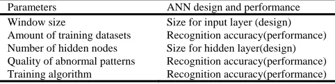
[image:1.612.308.549.459.520.2]

In this paper, full factorial DOE was utilized in investigating the effects of several parameters to the recognition accuracy of a three layer ANN. Then, an optimal ANN design was proposed. Table 1 shows the relationship of such parameters to the design and performance of an ANN.

Table 1. Relationship of parameters to an ANN

Parameters ANN design and performance Window size Size for input layer (design) Amount of training datasets Recognition accuracy(performance) Number of hidden nodes Size for hidden layer(design) Quality of abnormal patterns Recognition accuracy(performance) Training algorithm Recognition accuracy(performance)

2. Control chart patterns

CCPs were classified as normal and abnormal patterns (i.e. upward and downward shifts, upward and downward trends and cyclic). Ideally, data patterns should be tapped from real world. However, since a large number of data are needed, the simulated CCPs were developed using Monte Carlo simulation approach (see [12]). This methodology has been widely adopted in other researches [13]. Table 2 provides the parameters for simulating the abnormal CCPs.

(2)

[image:2.612.64.301.176.239.2]

were standardized to a range between [−3, +3] and then normalized to a compact range between [−1, +1]. For normalization, a maximum and a minimum values were taken once from the overall standardized samples. The normalization could minimize noise from the samples, thus provides an accurate and consistent recognition.

Table 2. Parameters for simulating abnormal patterns

Abnormal patterns

Range of magnitude (in σ)

Mag. intervals (coarse data)

Mag. intervals (fine data)

Upward shift 0.2 to 2.8 0.2, 0.4,… 0.2, 0.3,… Downward shift -2.8 to -0.2 -2.8, -2.6,… -2.8, -2.7,... Upward trend 0.015 to 0.025 0.015, 0.017, 0.015, 0.016,… Downward trend -0.025 to -0.015 -0.025,-0.023, -0.025,-0.024, Cyclic 0.5 to 2.5 0.5, 0.75,… 0.5, 0.6,…

3. Training and testing the recognizer

The performance of an ANN model was investigated in different back-propagation (BPN) training algorithms, i.e. (a) Levenberg-Marquardt (trainlm) and (b) Gradient descent with momentum and adaptive learning rate (traingdx). For ‘trainlm’, momentum constant and learning rate were set as 0.5, whereas maximum number of epochs and error goal were set as 500 and 0.001 respectively. For ‘traingdx’, learning rate and learning rate increment were set as 0.05 and 1.05, whereas maximum number of epochs and error goal were set as 1500 and 0.001 respectively.

[image:2.612.312.546.258.338.2] [image:2.612.312.552.527.642.2]

Network performance for both algorithms was based on mean square error (MSE). The hyperbolic tangent function in hidden layer limited the hidden output between [−1, +1] and sigmoid function in output layer limited the classification output between [0, 1].

The training process was stopped whenever either the error goal has been met or the maximum allowable training epoch has been reached. The ‘trainlm’ reached error goal between 15 and 40 epochs, while the ‘traingdx’ reach error goal between 100 to 300 epochs. In terms of time consuming, the ‘trainlm’ consumed longer time compared to the ‘traingdx’. It is because the ‘trainlm’ processed large data during training operation while the ‘traingdx’ processed small data.

The amount of training datasets was set as 400 and 800 for each pattern. Therefore, total training datasets for all patterns were 2400 and 4800. Then, 1000 datasets of each pattern were used for testing.

3.1. Output for patterns classification

Table 3 represents the target outputs for each CCPs. The maximum value (0.9) in each row identifies the

corresponding neuron expected to secure the highest output for correctly classified patterns.

The target output neuron (Ti) and the actual output neuron (Oi) were determined based on the maximum value produced from the six neurons. For instance, target values for normal and upward shift patterns were set as 0.9 at 1st and 2nd neurons respectively. If a normal pattern produced output as [0.7; 0.1; 0.1; 0.0; 0.3; 0.25], a maximum output was from the 1st neuron, thus a normal pattern was correctly classified. Inversely, if a normal pattern produced [0.3; 0.75; 0.1; 0.0; 0.3; 0.25], a maximum output was from the 2nd neuron, thus, the normal pattern was wrongly classified as upward shift pattern.

Table 3. A matrix of target outputs of an ANN

Target output in Oth_neuron

Patterns

O1 O2 O3 O4 O5 O6

Normal 0.9 0.1 0.1 0.1 0.1 0.1

Upward Shift 0.1 0.9 0.1 0.1 0.1 0.1 Downward Shift 0.1 0.1 0.9 0.1 0.1 0.1 Upward Trend 0.1 0.1 0.1 0.9 0.1 0.1 Downward Trend 0.1 0.1 0.1 0.1 0.9 0.1 Cyclic 0.1 0.1 0.1 0.1 0.1 0.9

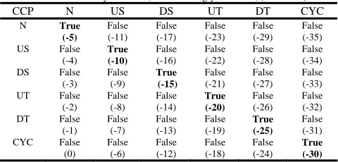
Outputs for CCPs that correctly classified and wrongly classified can be determined using the following equation:

Difference = (target neuron) – 6 x (actual output neuron)

where, 6 was a value based on the number of patterns categories. For examples, a normal pattern that correctly classified was computed as [1 – 6 ( 1 ) = –5], whereas a normal pattern that wrongly classified as upward shift was computed as [1 – 6 ( 2 ) = –11]. The overall ‘differences’ for the correctly classified and wrongly classified CCPs were arranged in Table 4.

Table 4. A matrix of correctly & wrongly classified CCPs

Note: True - correctly classified, False - wrongly classified, (difference) CCP N US DS UT DT CYC

N True (-5)

False (-11)

False (-17)

False (-23)

False (-29)

False (-35) US False

(-4)

True (-10)

False (-16)

False (-22)

False (-28)

False (-34) DS False

(-3)

False (-9)

True (-15)

False (-21)

False (-27)

False (-33) UT False

(-2)

False (-8)

False (-14)

True (-20)

False (-26)

False (-32) DT False

(-1)

False (-7)

False (-13)

False (-19)

True (-25)

False (-31) CYC False

(0)

False (-6)

False (-12)

False (-18)

False (-24)

True (-30)

4. Analysis and discussion

(3)

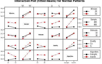
model analysis of variance (ANOVA). Percentage correct classification (recognition rate) for normal, upward shift, upward trend, and cyclic patterns were taken as the outcomes. The outcomes for downward shift were similar as for upward shift, whereas the outcomes for downward trend were similar as for upward trend. Table 5 to Table 8 show the results of ANOVA and Table 10 provides a design matrix and the DOE results. Figure 1 to Figure 4 represent the interaction effects among the investigated parameters.

4.1. The effects of each parameters

Window size has significant effects to an ANN accuracy in recognizing abnormal patterns but it has no effect for normal pattern. The interaction effects for shift, trend and cyclic patterns respectively presented the high recognition rate could be obtained at a large window size, i.e. 32. Generally, a small window size provided weak properties of abnormal patterns, while a large window size provided strong properties.

Guh and Tannock [6] proposed the selection of window size should balance between Type I error and

Type II error. It can be obtained by setting the ARLο≈

370, comparable to the Shewhart chart performance. Barghash and Santarisi [1], however, reported that window size has insignificant effect to Type I error

and Type II error in recognizing normal and shift patterns.

Winsize

99.0 97.5 96.0

Hidnode

Quality

Algorithm

trainlm traingdx

Sample

800

400 Co Fi

99.0 97.5 96.0 99.0

97.5 96.0

99.0 97.5 96.0

32 24 99.0 97.5 96.0

30 10

Winsize 24 32 Sample 400 800

Hidnode 10 30 Quality Co Fi Algorithm traingdx trainlm

[image:3.612.323.540.199.337.2]

Interaction Plot (fitted means) for Normal Patterns

Figure 1. Interaction effect plot for normal pattern

Table 5. ANOVA for recognizing normal pattern

Source DF Seq SS Adj SS Adj MS F P WS 1 6.081 6.081 6.081 2.42 0.123 TD 1 96.779 96.779 96.779 38.50 0.000 HN 1 1.069 1.069 1.069 0.43 0.516 QD 1 9.735 9.735 9.735 3.87 0.052 TA 1 98.526 98.526 98.526 39.20 0.000 WS*TD 1 1.877 1.877 1.877 0.75 0.389 WS*HN 1 1.877 1.877 1.877 0.75 0.389 WS*QD 1 17.331 17.331 17.331 6.90 0.010 WS*TA 1 28.785 28.785 28.785 11.45 0.001 TD*HN 1 8.456 8.456 8.456 3.36 0.069 TD*QD 1 5.569 5.569 5.569 2.22 0.139 TD*TA 1 75.799 75.799 75.799 30.16 0.000 HN*QD 1 9.191 9.191 9.191 3.66 0.058

HN*TA 1 0.439 0.439 0.439 0.17 0.677 QD*TA 1 9.735 9.735 9.735 3.87 0.052 --- Error 112 281.516 281.516 2.514

Total 127 652.767

S = 1.58541 R-Sq = 56.87% R-Sq(adj) = 51.10%

Amount of training datasets shows significant effects for normal, trend and cyclic patterns but shows insignificant effect for shift pattern. The interaction plots indicate that the large amount of training, i.e. 800 resulted in higher recognition accuracy.

Winsize

96 93 90

Hidnode

Quality

Algorithm

trainlm traingdx

Sample

800

400 Co Fi

96 93 90 96

93 90

96 93 90

32 24 96 93 90

30 10

Winsize 24 32

Sample 400 800 Hidnode 10 30 Quality Co Fi Algorithm traingdx trainlm

[image:3.612.312.539.358.524.2]

Interaction Plot (fitted means) for Upward Shift Patterns

Figure 2. Interaction effect plot for upward shift pattern

Table 6. ANOVA for recognizing upward shift pattern

Source DF Seq SS Adj SS Adj MS F P WS 1 655.13 655.13 655.13 187.14 0.000 TD 1 12.09 12.09 12.09 3.45 0.066 HN 1 0.19 0.19 0.19 0.05 0.816 QD 1 7.48 7.48 7.48 2.14 0.147 TA 1 933.44 933.44 933.44 266.64 0.000 WS*TD 1 2.24 2.24 2.24 0.64 0.425 WS*HN 1 4.51 4.51 4.51 1.29 0.259 WS*QD 1 58.35 58.35 58.35 16.67 0.000 WS*TA 1 47.56 47.56 47.56 13.58 0.000 TD*HN 1 25.15 25.15 25.15 7.18 0.008 TD*QD 1 92.17 92.17 92.17 26.33 0.000 TD*TA 1 2.51 2.51 2.51 0.72 0.399 HN*QD 1 3.36 3.36 3.36 0.96 0.329 HN*TA 1 51.28 51.28 51.28 14.65 0.000 QD*TA 1 5.37 5.37 5.37 1.53 0.218 --- Error 112 392.08 392.08 3.50

Total 127 2292.92

S = 1.87102 R-Sq = 82.90% R-Sq(adj) = 80.61%

Number of hidden node also provides significant effects in recognizing trend and cyclic patterns but provides insignificant effect for normal and shift patterns. Barghash and Santarisi [1] reported the number of hidden node has no effect to the Type I error and Type II error in recognizing normal and shift patterns respectively.

[image:3.612.79.296.422.559.2]

(4)

this parameter may indicate a non-linear trend to an ANN performance. Gauri and Chakraborty [14], for example, gave the results of non-linear recognition rate based on different numbers of hidden nodes.

Winsize

99.0 97.5 96.0

Hidnode

Quality

Algorithm

trainlm traingdx

Sample

800

400 Co Fi

99.0 97.5 96.0 99.0

97.5 96.0

99.0 97.5 96.0

32 24 99.0 97.5 96.0

30 10

Winsize 24 32 Sample 400 800 Hidnode 10 30 Quality Co Fi Algorithm traingdx trainlm

[image:4.612.78.294.123.265.2]

Interaction Plot (fitted means) for Upward Trend Patterns

[image:4.612.67.295.299.505.2]

Figure 3. Interaction effect plot for upward trend pattern

Table 7. ANOVA for recognizing upward trend pattern

Total 127 469.287

S = 1.02818 R-Sq = 74.77% R-Sq(adj) = 71.39%

Winsize

100.0 97.5 95.0

Hidnode

Quality

Algorithm

trainlm traingdx

Sample

800

400 Co Fi

100.0 97.5 95.0 100.0

97.5 95.0

100.0 97.5 95.0

32 24 100.0

97.5 95.0

30 10

Winsize 24 32

Sample 400 800 Hidnode 10 30 Quality Co Fi

Algorithm traingdx trainlm

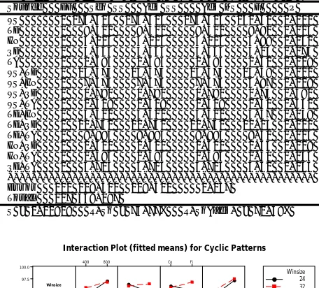
[image:4.612.78.295.459.609.2]

Interaction Plot (fitted means) for Cyclic Patterns

Figure 4. Interaction effect plot for cyclic pattern

Then, quality of abnormal patterns presented significant effect only for normal pattern. Abnormal patterns with fine quality data stream (small variation in magnitudes of abnormality) strengthened the abnormal patterns properties for better discriminating

from others CCPs. Inversely, abnormal patterns with coarse quality data stream (large variation in magnitudes of abnormality) have weak properties for discrimination. For example, shift pattern contain properties in terms of shift magnitudes, while trend pattern contain properties in terms of trend slopes.

The fifth parameter, i.e. training algorithm indicated significant effect for normal, shift and cyclic patterns. The interaction plots of such patterns show that the ‘trainlm’ algorithm resulted better recognition accuracy compared to the ‘traingdx’ algorithm.

Table 8. ANOVA for recognizing cyclic pattern

Total 127 924.072

S = 1.28404 R-Sq = 80.02% R-Sq(adj) = 77.34%

Based on the screening experiments, Table 9 summarizes the significant parameters associated to this study. Column 6th in Table 9 shows an optimal design selected for a three layers ANN recognizer, whereas run 12th in Table 10 provides the recognition rate achieved from an optimal ANN. Overall, this ANN model recognized 100% of normal patterns and 98.83% of abnormal patterns.

Table 9. Summary of the significant parameters

Note: √ - Significant (with better recognition accuracy); x – insignificant Design

Parameter

Normal Upshift Uptrend Cyclic Design selection WS x _√ (Large) √(Large) √ (Large) WS = 32 TD √ (Large) x _√(Large) √ (Large) TD = 800 HN x x _√(Small) √ (Small) HN = 10 QD √ (Fine) x _√ (Fine) x QD = Fine TA √(trainlm

)

√(trainlm )

x _√(trainlm )

TA=trainl m

5. Conclusion

[image:4.612.310.556.511.590.2]

(5)

empirically. This study, however, proved that the classical DOE can be utilized in designing ANNs by

screening the parameters that significantly influence the recognition accuracy of the ANNs.

6. References

[1] M.A. Barghash and N.S. Santarisi, “Pattern recognition of control charts using artificial neural networks – analysis the effects of the training parameters”, Journal of Intelligent Manufacturing, vol 15, pp. 635−644, 2004.

[2] F. Zorriassatine and J.D.T. Tannock, “A review of neural networks for statistical process control”,

Journal of Intelligent Manufacturing, vol. 9, no. 3, pp. 209−224, 1998.

[3] C.S. Cheng, “A multi-layer neural network model for detecting changes in the process mean”, Computers and Industrial Engineering, vol. 28, no. 1, pp. 51−61, 1995.

[4] C.S. Cheng, “A neural network approach for the analysis of control chart patterns”, International Journal of Production Research, vol. 35, no. 3, pp. 667−697, 1997.

[5] D.C. Reddy and K. Ghost, “Identification and interpretation of manufacturing process patterns through neural networks”, Mathematical Comput. Modelling, vol. 27, no. 5, pp. 15−36, 1998.

[6] R.S. Guh and J.D.T. Tannock, “Recognition of control chart concurrent patterns using a neural network approach”, International Journal of Production Research, vol. 37, no. 8, pp. 1743−1765, 1999.

[7] R.S. Guh and Y.C. Hsieh, “A neural network based model for abnormal pattern recognition of control charts”, Computers and Industrial Engineering, vol. 36, pp. 97−108, 1999.

[8] D.T. Pham and S. Sagiroglu, “Training multilayered perceptrons for pattern recognition: a comparative study of four training algorithms”, International Journal of Machine Tools & Manufacture, vol. 41, pp. 419−430, 2001.

[9] R.S. Guh, F. Zoriassatine, J.D.T. Tannock, & C. O’Brien, “On-line control chart pattern detection and discrimination – a neural network approach”. Artificial Intelligence in Engineering, vol. 13, pp. 413-425, 1999.

[10] S.K. Gauri & S. Chakraborty, “Feature-based recognition of control chart patterns”. Computers and Industrial Engineering, vol. 51, pp. 726-742, 2006.

[11] A. Hassan, M.S. Nabi Baksh, A.M. Shaharoun, and H. Jamaluddin, “Feature selection for SPC chart pattern recognition using fractional factorial experimental design”, 2nd I*IPROMS Virtual International Conference on Intelligent Production Machines and Systems, 3−14 July 2006.

[12] J.A. Swift, “Development of a Knowledge Based Expert System for Control Chart Pattern Recognition and Analysis”, Ph.D Dissertation, Oklahoma State University.

[13] A. Hassan and M.S. Nabi Baksh, “Recognition of developing SPC chart patterns using ANN and stability tests”, International Symposium on

Bio-Inspired Computing, September 2005, Putri Pan

Pacific Hotel, Johor Bahru, Malaysia.

(6)

[image:6.612.54.564.135.708.2]

7. Appendix

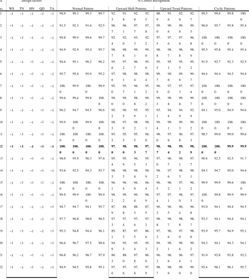
Table 10. Design matrix and results for full factorial design of experiments

Ru n

Design factors % Correct Recognition

no. WS TN HN QD TA Normal Pattern Upward Shift Patterns Upward Trend Patterns Cyclic Patterns 1 ₋1 ₋1 ₋1 ₋1 ₋1 98.9 99.3 99.3 99.7 92.

3 91. 8 92. 6 92. 5 88. 9 91. 6 92. 6 92. 7

99.5 99.6 99.8 100.

0

2 +1 ₋1 −1 −1 −1 91.5 92.3 91.6 92.5 96. 7 96. 1 97. 7 97. 8 99. 0 99. 6 99. 6 99. 5

96.0 95.7 95.8 95.4

3 ₋1 +1 ₋1 −1 −1 99.8 99.9 99.6 99.7 92. 4 92. 0 93. 3 92. 2 97. 5 97. 6 97. 6 96. 8 100. 0 100. 0 100. 0 100. 0

4 +1 +1 ₋1 −1 −1 94.9 92.9 95.4 95.7 98. 7 98. 8 99. 1 99. 0 98. 8 98. 7 98. 8 98. 9

95.5 95.8 95.4 95.4

5 ₋1 −1 +1 ₋1 −1 94.6 95.1 96.2 96.2 95.

6 97. 2 96. 7 95. 6 95. 5 95. 1 95. 5 95. 2

91.9 92.7 92.3 92.5

6 +1 ₋1 +1 ₋1 −1 95.7 95.6 95.9 95.2 97.

6 98. 1 98. 4 98. 4 99. 7 99. 6 99. 6 99. 7

94.4 94.4 94.5 94.4

7 ₋1 +1 +1 ₋1 −1 100.

0 99.9 100. 0 99.9 95. 0 95. 7 96. 1 95. 2 96. 9 97. 0 97. 3 97. 4 100. 0 100. 0 100. 0 100. 0

8 +1 +1 +1 ₋1 −1 99.6 99.4 99.8 100.

0 99. 0 99. 0 98. 8 99. 2 99. 3 99. 8 99. 8 99. 7 100. 0 100. 0 100. 0 100. 0

9 ₋1 −1 −1 +1 ₋1 96.2 94.7 94.5 96.6 95.

2 96. 5 95. 9 95. 1 93. 1 94. 4 94. 9 93. 9

94.1 95.0 94.9 94.6

10 +1 ₋1 −1 +1 ₋1 99.9 100.

0 99.9 100. 0 98. 3 97. 9 98. 2 98. 1 99. 4 99. 1 99. 3 99. 2 100. 0 100. 0 100. 0 100. 0

11 ₋1 +1 ₋1 +1 ₋1 100.

0 100. 0 100. 0 100. 0 95. 2 95. 5 95. 5 96. 0 98. 0 97. 6 96. 8 97. 3

98.7 99.0 99.0 99.6

12 +1 +1 ₋1 +1 ₋1 100. 0 100. 0 100. 0 100. 0 97. 0 98. 0 98. 3 97. 7 98. 7 98. 4 99. 2 98. 9 100. 0 100. 0 99.9 99.9

13 ₋1 −1 +1 +1 ₋1 96.0 95.9 96.3 97.6 95. 4 95. 9 96. 5 95. 3 97. 0 96. 7 98. 1 97. 7

90.4 92.5 92.5 91.7

14 +1 ₋1 +1 +1 ₋1 93.6 92.5 94.3 93.7 98. 3 98. 3 98. 6 98. 9 98. 2 97. 6 98. 3 98. 1

94.3 94.7 95.0 94.4

15 ₋1 +1 +1 +1 ₋1 100.

0 100. 0 100. 0 100. 0 96. 1 96. 4 96. 9 96. 4 96. 5 96. 2 97. 1 96. 2

99.9 99.9 99.6 100.

0

16 +1 +1 +1 +1 ₋1 99.9 99.9 100.

0 99.9 98. 2 99. 2 99. 4 98. 9 97. 4 97. 1 98. 0 97. 3 100. 0

99.8 99.9 99.9

17 ₋1 −1 −1 −1 +1 94.7 94.7 94.1 95.7 87.

9 88. 8 88. 3 87. 5 96. 3 96. 5 96. 4 96. 8

93.0 94.1 94.4 94.5

18 +1 ₋1 −1 −1 +1 97.7 96.8 98.0 96.5 97.

3 97. 4 97. 6 97. 2 98. 8 98. 7 98. 8 98. 7

93.3 94.1 94.4 94.1

19 ₋1 +1 ₋1 −1 +1 95.3 94.8 94.4 96.1 85.

1 87. 3 87. 5 86. 6 97. 2 96. 6 97. 0 98. 0

93.9 95.7 94.9 95.1

20 +1 +1 ₋1 −1 +1 96.6 96.7 97.5 98.6 94.

9 95. 3 95. 4 95. 3 99. 2 99. 1 99. 6 99. 2

94.3 94.1 94.3 94.1

21 ₋1 −1 +1 ₋1 +1 96.8 96.2 96.7 97.9 86.

3 88. 0 87. 8 86. 0 96. 3 96. 6 96. 4 97. 1

91.0 92.8 92.8 92.2

22 +1 ₋1 +1 ₋1 +1 94.9 94.5 95.8 95.1 97. 6 97. 6 97. 8 97. 9 98. 7 98. 6 99. 0 99. 0

(7)

23 ₋1 +1 +1 ₋1 +1 94.9 94.3 94.8 96.1 87. 1

88.

7 88.

5 87.

3 97.

4 97.

1 96.

8 97.

3

94.0 94.8 94.4 95.2

24 +1 +1 +1 ₋1 +1 94.7 94.5 96.1 96.1 90. 5

89.

9 89.

4 89.

2 99.

3 99.

0 99.

2 98.

9

95.0 96.2 95.6 95.0

25 ₋1 −1 −1 +1 +1 95.0 94.3 94.9 95.5 87.

7 90.

6 88.

9 88.

3 96.

4 96.

3 96.

2 96.

4

93.6 95.3 94.6 94.4

26 +1 ₋1 −1 +1 +1 95.5 95.1 96.5 97.1 88.

0 87.

3 88.

0 87.

8 98.

6 99.

0 99.

2

94.0 94.6 94.4 94.3

27 ₋1 +1 ₋1 +1 +1 96.3 95.3 95.4 97.0 91.

5 93.

4 92.

3 91.

3 94.

7 94.

0 94.

7

92.8 94.7 94.1 94.5

28 +1 +1 ₋1 +1 +1 96.4 96.0 96.9 97.0 98.

1 98.

9 99.

1 98.

6 98.

9 98.

3 99.

2 98.

9

94.3 94.5 95.0 94.7

29 ₋1 −1 +1 +1 +1 96.8 95.7 95.5 97.1 87.

0 89.

3 88.

3 87.

8 95.

3 95.

5 95.

1 95.

6

91.8 93.7 93.7 93.0

30 +1 ₋1 +1 +1 +1 94.6 93.7 95.9 95.1 92.

4 91.

3 90.

8 91.

4 99.

5 99.

3 99.

4 99.

4

95.6 96.2 95.7 95.5

31 ₋1 +1 +1 +1 +1 96.1 94.7 95.2 97.1 87. 4

89.

5 88.

0 88.

4 96.

1 95.

7 95.

7 96.

3

93.2 95.0 94.0 93.8

32 +1 +1 +1 +1 +1 96.5 95.6 96.8 97.0 94.

5 95.

3 95.

1 95.

1 99.

1 98.

6 99.

0 99.

0