A Novel Floating Point Fast Confluence Adaptive
Independent Component Analysis for Signal Processing
Applications
Jayasanthi Ranjith. M.E.
1, NJR.Muniraj
21Anna University, Tamil nadu,India
2Principal,Tejaa Sakthi Institute of Technology for Women,Tamil Nadu, India *Corresponding Author: [email protected]
Copyright © 2013 Horizon Research Publishing All rights reserved.
Abstract
Independent component analysis (ICA) is a technique that separates the independent source signals from their mixtures by minimizing the statistical dependence between components. This paper presents a floating point implementation of a novel fast confluence adaptive independent component analysis (FCAICA) technique with reduced number of iterations that provides the high convergence speed. Fixed point ICA algorithms cover only smaller range of numbers. To handle large as well as tiny numbers and hence to improve the dynamic range of the signal values,floating point operations are performed in ICA. The high convergence speed is achieved by a novel optimization scheme that adaptively changes the weight vector based on the kurtosis value. To validate the performance of the proposed FCAICA, simulation and synthesis are performed with super-gaussian mixtures and sub Gaussian mixtures and experimental results provided. The proposed FCAICA processor separates the super-Gaussian signals with a maximum operating frequency of 2.91MHz with improved convergence speed.Keywords
Adaptive Independent Component Analysis, Blind Source Separation, Contrast Function Optimization, Field Programmable Gate Array, Floating Point Independent Component Analysis, Very Large Scale Integration1. Introduction
ICA, a statistical signal processing technique, is one of the most commonly used algorithms in blind source separation. The term “blind” means that both the original independent sources and the way the sources were mixed are all unknown. Estimates of the source signals are found only from the observed signal mixtures. ICA recovers source signals from their mixtures by finding a linear transformation that maximizes the mutual independence or non-gaussianity of
correlation matrix [10]. A frequency-domain method of blind source separation (FD-BSS) is able to separate acoustic sources under highly reverberant challenging conditions [11]. In frequency-domain BSS, the separation is generally performed by applying ICA at each frequency envelope. ICA is also done by entropy bound minimization (ICA-EBM) [12].
Fixed-point VLSI architecture was proposed for 2-Dimensional Kurtotic FastICA with reduced and optimized arithmetic units [13]. Implementation of the ICA algorithm on a fixed point platform and floating point processor shows that the accuracy and speed of the fixed point platform were found to be acceptable. In addition, the fixed point processor needs less space and consumes less power. But fixed point processor can handle only smaller range of real values [14]. Due to the computation complexities and convergence rates, ICA is very time-consuming for high volume or high dimensional data set like hyperspectral images. In Parallel ICA (pICA), ICA module is partitioned into three temporally independent functional modules, and each of them is synthesized individually. All these modules are developed for reuse and retargeting purpose. It provides an optimal parallelism environment, a potential faster and real-time solution [15]. FPGA implementation of ICA in digital chip is reported with the modular design concept in [16] and with systolic architecture in [17]. A mixed-signal VLSI system that operates on spatial and temporal differences in the acoustic field at very small aperture to separate and localize mixtures of traveling wave sources is presented in [18].
Evolutionary computation techniques which are population search based optimization methods like genetic algorithms and Particle swarm optimization are used in ICA [19][20] [21]. The only disadvantage of evolutionary computation based ICA technique is that it has heavy computational complexity. But with the advent of highly parallel processors and new technologies like VLSI, these methods provide competitive solutions to the problems.
Though current speech-recognition technologies are quite successful for clean speech signals, their performance is poor in real-world noisy environment which prevents it from becoming popular. Speech enhancement techniques to be made to overcome this difficulty are adaptive noise canceling (ANC) and blind signal separation (BSS). ANC reduces noise when there is knowledge of reference noise signals. When no reference signal is known, then the problem is the BSS problem [23]. ICA technique is mostly used in BSS problems. Two different ICA methods named as Shuffled Frog Leap optimization based ICA and Fast Confluence Adaptive ICA are proposed in floating point arithmetic in this paper. Most commonly used Fast ICA algorithm that provides high convergence speed is also developed for comparison purpose. In order to enable the real-time ICA processing in VLSI and to speed up the computation, the ICA algorithms are written by hand coding HDL code. Various analog VLSI implementations of ICA also exist in the literature. Since digital adaptation offers the
flexibility of reconfigurable ICA learning rules, digital implementations are common practice in this field. Though there is software that translates the high-level languages such as C code, MATLAB, and even Simulink into HDL code, hand coding gives the power optimized Implementation with improved performance.
The originality of the proposed FCA ICA is summarized as follows:
The early determination of converging weight vector and demixing matrix reduces the number of
operations and hence the power consumption.
Convergent speed is improved by changing the weight vectors according to fitness value.
Floating point arithmetic improves the precision and dynamic range of the signals.
This paper is organized as follows. Section II describes the background of ICA. Section III presents the implementation of the FP arithmetic units. Section IV describes the FastICA algorithm. Section V describes proposed SFLO optimization algorithms for ICA that is based on evolutionary algorithms. Section VI describes proposed FCA ICA and Section VII demonstrates the simulation and implementation results. Finally, conclusions are drawn in Section VIII.
2. Background of ICA
A long-standing problem in statistics and related areas is to find a suitable representation of multivariate data. Representation here means that data is transformed so that its hidden, essential structure is made more visible or accessible. Blind source separation is a problem of finding a linear representation of hidden data from the mixture in which the components are statistically independent. In practical situations, we cannot in general find a representation where the components are really independent, but we can at least find components that are as independent as possible. Independent component analysis is a major task in signal processing to extract the source signals from the observed mixtures. The relationship between source signals S and observed mixtures X is given in matrix notation as in (1).
X = A S (1) A is a full rank matrix which is called mixing matrix. Under some assumptions, ICA solves the BSS problem by finding inverse linear transformation such that, it maximizes the statistical independence between the observed mixtures. In doing this, ICA finds unmixing matrix B. Then the estimate of the source signal (S_est) is found from (2)
S_est= B X=S (2)
2.1. ICA Preprocessing
mixed signal involves finding the mixing matrix P. The first step in preprocessing is called centering.
Figure 1. Implementation of Centering
Let N statistically independent sources be mixed through NxN nonsingular mixing matrix A so that we obtain the observed signal mixtures given by x1(t),x2(t)..xn(t) which are the amplitudes of the recorded signals at time point t . For N=2, representation of original source signals is given by s1(t),s2(t) and mixtures are x1(t) and x2(t). Centering consists of subtracting the mean from each observed mixtures X1(t) and X2(t) to produce zero mean outputs C_X1 and C_X2 as shown in Fig.1.
Figure 2. Implementation Of Whitening
The second step is called Whitening and consists in linear transformation of the centered mixtures, to obtain new vectors which are white. Fig.2 shows the whitening process. The components of a whitened vector are uncorrelated and their variances equals to unity. This means that the covariance matrix of whitened data is equal to the identity matrix. One way to perform whitening is to use Eigen value Decomposition (EVD). The whitening matrix can be found by using (6)
P = ED-1/2 ET (6) Where E is the orthogonal matrix of eigenvector found from the covariance matrix E {XXT}.D is the diagonal matrix of the eigenvalues associated with each eigenvector.
The efficiency of ICA is based on the selection of cost functions, also called objective functions or contrast functions. The Cost function in some way or other is a measure of independence [2]. Some measures of independence are Kurtosis, negentropy and mutual information. Though there are different contrast functions, the most popular contrast function used in ICA is kurtosis.
3. Floating Point Arithmetic
Based on the storage area available, there are two variants
[image:3.595.316.549.146.197.2]of floating point representation of a real number i.e. IEEE single-precision representation and IEEE double-precision representation. IEEE single precision format, that uses 32 bits, has been used for this proposed ICA algorithm. Format of 32 bit Floating Point Representation is shown in Fig 3.
Figure 3. 32 bit Floating Point Format Representation
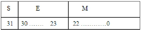
The sign field S in Fig. 1 is used to specify the sign of the real number. Exponent field E is a 8 bit quantity represented by using a bias of 127. Bits 22 down to 0 in field M are used to store the binary representation of the floating point number. Since leading one in the mantissa is implicit, it does not appear in the representation. Addition, subtraction, multiplication, division and square root operations are carried out following the appropriate algorithms of single precision IEEE 754 standard [31].
4. Fast ICA
4.1. The Fast ICA Algorithm
Due to simplicity and fast convergence, Fast ICA is considered as one of the most popular solutions for linear ICA/BSS problem .The VLSI implementation of this algorithm involves the preprocessing discussed in chapter II and iteration scheme.
4.1.1 Iteration for One Unit
The fast ICA algorithm for one unit estimates one row of the demixing matrix as a vector that is an extremum of contrast functions. Fast ICA is an iterative algorithm, derived from kurtosis based contrast function. Assuming Z as the whitened data vector and
w
T(
k
+
1
)
as one of the rows of the separating matrix,estimation ofw
T(
k
+
1
)
is done iteratively until convergence is achieved. The Fast ICA algorithm involves the following steps. Choose an initial random vector of unit norm (wold ).
Find norm of vectors and divide by corresponding norms.
Update the frog by the formula using whitened data vector Z to find wnew
3
{ ( ( )
T) } 3 ( )
new
w
=
E Z w k Z
−
w k
If wnew-wold < ε is not satisfied then go back to step 2. where ε is a convergence parameter (~10-4) and wold is the value of before it‘s replacement by the newly calculated value wnew.
4.1.2. Fixed-Point Iteration for Finding Several ICs
[image:3.595.59.295.331.423.2]using a deflationary approach one by one or estimated simultaneously by symmetric approach.In order to prevent that the algorithm estimates the same component more than one time, the orthogonalization is made using (3) and (4). This verification is done by subtracting the projections of all previously estimated vectors from the current estimate after every iteration step and before normalization.
j j T p p
p
w
w
w
w
w
(
−
(
)
(3) In the symmetric approach the iteration step is computed for all wp and the matrix W is orthogonalized asw
ww
w
←
(
T)
−
1
/
2
(4)The results are obtained in Fast ICA following the deflationary approach.
5. SFLO ICA
In this ICA method, contrast function optimization is performed based on SFLO for improving the optimality and convergence performance. Mutation operator introduced in SFLO Algorithm avoids the solution from getting trapped in local minima. It converges better in lesser time when compared to other optimization algorithms. In this algorithm, initial weight vectors for estimating the demixing matrix are assumed as frogs and updated by step 3 of the algorithm. Then fitness value is calculated and sorting is done according to fitness value. Based on the fitness values, total population is partitioned into q groups (memeplexes) of p frogs,that search independently. In this process, the first frog goes to the first memeplex, the second frog goes to the second memeplex, frog p goes to the pth memeplex, and frog p +1 goes back to the first memeplex and so on. In each memeplex, the frogs with the best and the worst fitnesses are identified as Xb and Xw , respectively. Also, the frog with the most qualified fitness level among all the memeplexes is identified as Xg. Then improvement is done to improve only the frog with the worst fitness according to step (8). If this process produces a better solution, it replaces the worst frog. Otherwise, a new population is randomly generated to replace that population. This process continues for a specific number of iterations (Imax1).Then all memeplexes are combined and sorted. Then mutation operation is included using (11) to avoid local minima. If the current iteration number reaches (Imax2), the search procedure is stopped; otherwise it goes to Step 5. The last Xg is the solution of the problem.
5. 1. Floating Point Iteration
Estimation of
w
T(
k
+
1
)
is done iteratively with following steps until a convergence is achieved. Choose initial population of ‘n’ frogs (weights) at random.
Find norm of pair of frogs and divide by corresponding norms.
Update the frogs by the formula
) ( 3 } ) ) ( ( { ) 1
(k E Z w k Z 3 w k
w + ← T −
Calculate the fitness value from
)
(
)
1
(
k
w
k
w
f
=
+
−
Sort the initial population based on the fitness values with decreasing manner.
Partition the sorted population into p memeplexes of q frogs.
Select the best frog (Xb), worst frog (Xw) in each memeplex and globally best frog (Xg).
Update the position of Xw using Xw(new) =Xw(old) +C.
where C= rand( ).(Xb-Xw).
If it produces better solution, older frog is replaced by updated frog and this process continues for a specific number of iterations (Imax1). Otherwise a new frog is randomly generated to replace Xw and algorithm goes to step 2.
All memeplexes are combined and sorted again.
Apply mutation
(.)(
)
(.)(
)
i i i i i i
mut rand b rand g rand
X
=
X
+
rand X X
−
+
rand X X
−
If the current iteration number reaches Imax2, the search procedure is stopped or it goes to Step 5.
The last X g is the solution of the problem. Here i
rand
X
is a randomly generated vector, Nmem is the number of memeplexs, i=1,2,……Nmem ,rand
(.)
is random number between (0 and 1) and ε is a convergence parameter (~10-4). With the above steps, Deflationary othogonalization is made to find second independent component.6. Novel Floating Point Fast Confluence
Adaptive ICA
Though the above algorithm which is based on SFLO improves the optimality performance, it suffers from computational complexity due to large number of iterative calculations in floating point iteration scheme. For reducing the number of manipulations and for improving the performance of ICA algorithm in terms of convergence speed, adaptive optimization of contrast function is proposed in floating point arithmetic. Here, initial weight vectors for estimating the demixing matrix B in (2), are assumed as frogs and are described as memetic vectors. This algorithm computes new weights (frogs) from the initial weights in adaptive manner based on fitness value.
6.1. Floating Point Iteration for One Unit
of weights continues in iterative manner with following steps until a convergence is achieved.
Choose initial frogs (wi) of ‘N’ numbers at random.
Find norm of frogs and divide by corresponding norms.
Update all the N frogs by using the formula ) ( 3 } ) ) ( ( { ) 1
(k E Z w k Z 3 w k
w + ← T −
Calculate the fitness value
)
(
)
1
(
k
w
k
w
f
=
+
−
and sort the frogs according to the fitness values. Divide the N frogs into M groups (N=2*M) with 2 frogs in each group. The division is done in such a way that 1st frog goes to 1st group, 2nd frog goes to 2nd group and continuous up to M frogs. Then (M+1)th frog goes to 1st group and so on.
In each group, determine the best and worst individuals. Update the worst frogs using step 3.
If
{
w
(
k
+
1
)
−
w
(
k
)}
<
ε
is not satisfied, then go back to step 2 by adaptively taking a new ‘wi’ lesserthan that of worst frog where ε is a convergence parameter (~10-4).
When
{
w
(
k
+
1
)
−
w
(
k
)}
<
ε
is satisfied, move to next group of frogs and repeat from step 6 until Iteration limit is reached.Then the two vectors with good fitness value can be used as row vectors of demixing matrix. With the above steps, Deflationary othogonalization is then made to find second independent component.
7. Results and Discussion
For verification of the validity and performance of the Fast ICA and the two proposed ICA algorithms, two different sub Gaussian and super-gaussian signal mixtures are taken and applied to the algorithms. The original signals are mixed with artificial mixing matrix A. The mixing matrix is a full rank matrix of 2 rows and 2 columns. The experiment was carried out first, for small-sized problem with 256 samples. Because the defined algorithm must be capable of efficiently solving the real-world sized instances, another experiment is carried out for large-sized problem with 3000 samples each.
[image:5.595.313.551.140.389.2]7.1. Simulation Results of ICA Algorithms
Table 1. Convergence Speed of ICA algorithms Parameters/
Algorithms Fast ICA SFLO-ICA FCA-ICA Convergence
Time T (ps) 300 500 200
The algorithms are written in VHDL and the simulation results are obtained from Modelsim 10.0c Tool. Table 1 compares the performance of Fast ICA, SFLO ICA and FCA-ICA in terms of convergence speed T. Here T represents the time taken for each of the algorithms to reach
convergence. The FCA-ICA based extraction of components from their mixtures possesses faster convergence compared to other two.
7.2. Results of Supergaussian Mixture
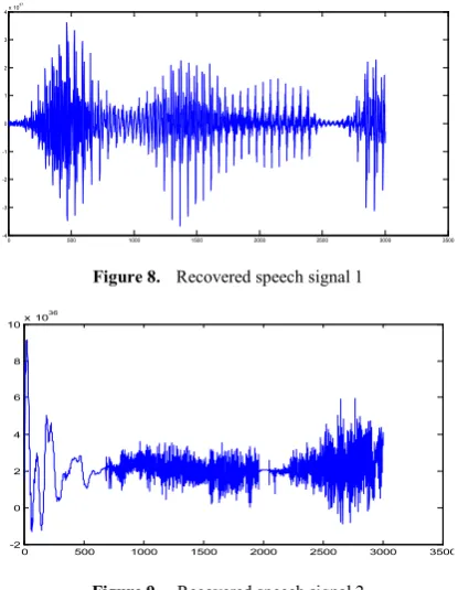
Figure 4. Speech signal 1
Figure 5. Speech signal 2
[image:5.595.317.550.484.737.2]The original speech signals obtained are shown in Fig 4 and Fig.5 respectively. Supergaussian signals have kurtosis value greater than zero. Examples of supergaussian signals are Speech signal, Train sound, Car noise etc. The super-gaussian mixture signals are shown in Fig 6 and 7 respectively. Fig.8 and Fig 9 shows the independent components obtained through proposed systems.
Figure 6. Mixture of speech signal 1
Figure 7. Mixture of speech signal 2
0 500 1000 1500 2000 2500 3000 3500
-0.4 -0.3 -0.2 -0.1 0 0.1 0.2 0.3 0.4
0 500 1000 1500 2000 2500 3000 3500
-0.02 0 0.02 0.04 0.06 0.08 0.1
0 500 1000 1500 2000 2500 3000 3500
-2 -1.5 -1 -0.5 0 0.5 1 1.5 2
0 500 1000 1500 2000 2500 3000 3500
[image:5.595.59.297.635.688.2]Figure 8. Recovered speech signal 1
Figure 9. Recovered speech signal 2
7.3. Results of Subgaussian Mixture
Subgaussian signals have kurtosis value lesser than zero. When kurtosis is zero, the signal is Gaussian for which ICA cannot be applied. Sine waves, sawtooth waves are examples of subgaussian signals. Two signals as in (5) and (6) each are taken and instantaneously mixed by the artificial mixing matrix A shown in (14)
S1=sin(2*pi*50*t) (5) S2=square(2*pi*50*t) (6)
Figure 10. Sine Wave Mixed With Matrix A
Figue 11. Square Wave Mixed With Matrix A
[image:6.595.321.543.122.402.2]The subgaussian mixture signals are shown in Fig 10 and 11 respectively. Fig.12 and Fig 13 shows the independent components obtained through proposed systems
Figure 12. Recovered sine wave
Figure 13. Recovered square wave
8. Conclusion
In this paper, new time-domain approaches to estimate the independent components of from observed super Gaussian and sub-gaussian mixtures have been presented. Use of modularity and hierarchy simplifies the design, reduces the area and speeds up the convergence process of ICA. The usage of optimization algorithm enables finding optimal solutions. Floating point manipulations enable increased input signal range. The peculiarity of the resulting system is the capability of providing faster convergence with reduced power. Further research includes the application of the proposed method for other signals, such as Electroencephalograph (EEG), Spread spectrum signals and images under poor Signal to noise ratio (SNR) circumstances. Further improvement is possible by employing this technique with more than two sources. The FCA ICA, Fast ICA and SFLO ICA (Shuffle Frog Leap Optimization based ICA) algorithms converge to the optimal solution at 300ps, 200ps and 500ps respectively.
REFERENCES
[1] E. Oja and Z. Yuan, “The FastICA Algorithm Revisited: Convergence Analysis”, IEEE Trans. Neural Networks, vol.
0 500 1000 1500 2000 2500 3000 3500
-4 -3 -2 -1 0 1 2 3 4x 10
37
0 500 1000 1500 2000 2500 3000 3500
-2 0 2 4 6 8 10x 10
36
0 50 100 150 200 250 300
-1 -0.8 -0.6 -0.4 -0.2 0 0.2 0.4 0.6 0.8 1
0 50 100 150 200 250 300
-1 -0.8 -0.6 -0.4 -0.2 0 0.2 0.4 0.6 0.8 1
0 50 100 150 200 250 300
-8 -6 -4 -2 0 2 4 6 8x 10
38
0 50 100 150 200 250 300
-8 -6 -4 -2 0 2 4 6 8x 10
[image:6.595.78.294.464.738.2]17, no. 6, November,2006.
[2] Hyvärinen, J. Karhunen, and E. Oja, “Independent Component Analysis”.New York: Wiley, 2001.
[3] T.Yamaguchi, I. Kuzuyoshi., “An Algebraic Solution to Independent Component Analysis”, Optics Communications, Elsevier Science, 178, pp.59-64, 2000.
[4] A.J.Bell and T.J.Sejnowski ”An information-maximization approach to blind separation and blind decovolution”, Neural Computation, 7, pp.1129-1159, 1995.
[5] A.Cichocki et al.,”Robust Neural Networks with on line biasing for blind identification and blind source separation” IEEE Trans. On Circuits and Systems, vol-43, no.11, pp.894-906, 1996.
[6] E.Oja,”Nonlinear PCA criterion and maximum likelihood in independent component analysis”, Proc. Int. Workshop on Independent Component Analysis and Signal separation (ICA’99), pp.143-148, Aussois, France, 1999.
[7] A.Hyverinen and E.Oja,”Independent component analysis by general nonlinear Hebbian like learning rates”, Signal Processing, vol-64, No.3, pp.301-303, 1998.
[8] F. Herrmann and A. K. Nandi”Maximisation of squared cumulants for blind source separation” Electronics Letters, 36(19), pp.1664–1665, 1996.
[9] K. Nandi and V. Zarzoso,” Fourth-order cumulant based blind source separation” IEEE Signal Processing Letters, 3(12), pp.312–314, 1996
[10] J.F.Cardoso ,”Source separation using higher order moments” Proc. of the IEEE Int. Conf on Acoustics, Speech and Signal Processing (ICASSP 1989), pp. 2109–2112, Glasgow, UK, May 1989.
[11] Francesco Nesta, Piergiorgio Svaizer, and Maurizio Omologo,”Convolutive BSS of Short Mixtures by ICA Recursively Regularized Across Frequencies” , IEEE Trans. Audio, Speech, And Language Processing, Vol. 19, No. 3, March 2011
[12] Xi-Lin Li and Tülay Adali,”Independent Component Analysis by Entropy Bound Minimization”, IEEE Trans. Signal Processing, Vol. 58, No. 10, October 2010
[13] Amit Acharyya, Koushik Maharatna,”Hardware Efficient Fixed-Point VLSI Architecture for 2D Kurtotic
FastICA”,IEEE 2009
[14] Dinesh Patil, Niva Das1, Aurobinda
Routray2 ,”Implementation of Fast-ICA: A Performance Based Comparison Between Floating Point and Fixed Point DSP Platform”, Measurement Science Review, Volume 11, No. 4, 2011
[15] Hongtao Du and Hairong Qi,” A Reconfigurable FPGA System for Parallel Independent Component Analysis”. EURASIP Journal on Embedded Systems, Volume 2006, Article ID 23025, Pages 1–12
[16] Abdullah Celik, Milutin Stanacevic and Gert Cauwenberghs,”Gradient Flow Independent Component Analysis in Micropower VLSI”.
[17] H. Jeong, Y. Kim, H. J. Jang,” Adaptive Parallel Computation for Blind Source Separation with Systolic Architecture”, Intelligent Information Management, 2010, 2, 46-52
[18] Hongtao Du, Hairong Qi and Xiaoling Wang,” Comparative Study of VLSI Solutions to Independent Component Analysis” IEEE Trans. Industrial Electronics, VOL. 54, NO. 1, FEBRUARY 2007
[19] F.Rojas, C.G.Puntonet, M.Rodriguez-Alvarez, I.Rojas, and R.Martin-Clemente, “Blind Source separation in post-nonlinear mixtures using competitive learning, simulated annealing and a genetic algorithm” IEEE Trans. On Systems, Man and Cybernatics –Part C: Applications and Reviews, vol.34, no.4, pp.407-416, Nov. 2004.
[20] R.Palaniappan and C.N.Gupta, Genetic Algorithm based independent component analysis to separate noise from Electrocardiogram signals, Proc. IEEE, 2006.
[21] D. J. Krusienski and W. K. Jenkins,”Nonparametric Density Estimation Based Independent Component Analysis via Particle Swarm Optimization”, Proc. IEEE, pp. IV – 357- IV – 360, 2005.
[22] Alan Paulo , Ana Maria ,”FPGA hardware design, simulation and synthesis for a Independent component analysis algorithm using system-level design software”.